My Account     Contact Us     Cart

Mapping Class: Work with Sentinel-2 Imagery in Geographic Imager – Part Two, with Tom Patterson

***

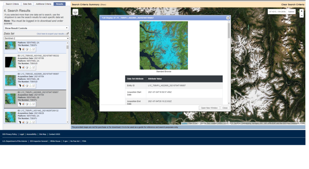
Welcome back to Mapping Class! The Mapping Class tutorial series curates demonstrations and workflows created by professional cartographers and expert Avenza software users. Today Tom Patterson is sharing with us part two of his demonstration of editing Sentinel-2 Imagery Data using Geographic Imager and Adobe Photoshop. Continued from Part One, Tom shows how to take his newly crafted true-color image to make water regions really pop! He will show you how you can use the mosaic tool in Geographic Imager to work with elevation data to create layer masks that make adjusting water areas easy.

If you missed last month’s edition of Mapping Class, check out Part One of Tom’s demonstration.

We have also compiled supplementary video notes below.

***

Work with Sentinel-2 Imagery in Geographic Imager: Part Two
by Tom Patterson (Video notes adapted from original)

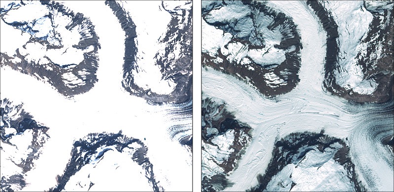
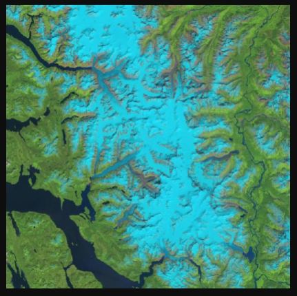
The vegetation brightening technique from part one also influences the color of water bodies. In part two, we will shift water bodies to a more attractive blue and diminish reflections, wind riffles, and sediment plumes. The technique involves adding a flat blue layer with an accompanying water layer mask in Photoshop.

Create a Water-Layer Mask

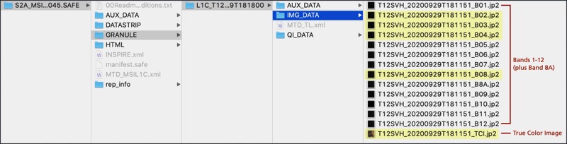
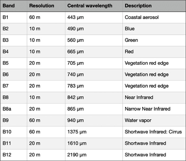
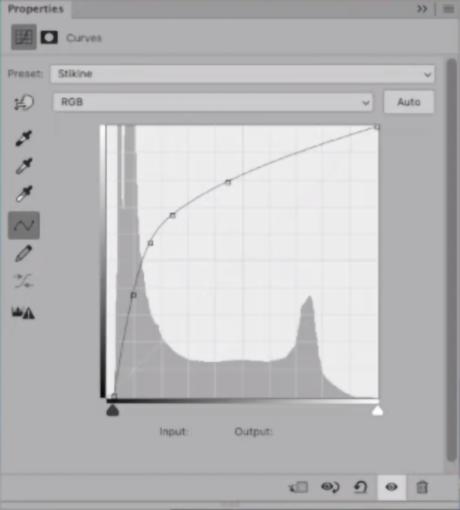
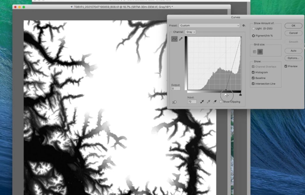
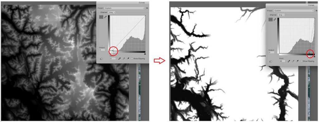
We will create the water layer mask from band 8. It contains data from the near-infrared section of the spectrum that clearly delineates water and land areas. Applying a steep curves adjustment to band 8 will compress the tonal range, which when inverted, results in a high-contrast land-water mask.

The trick is to adjust the curve in such a way so that it minimizes blemishes in the water and shadows on the land. Unfortunately, with this dataset, mountain cast shadows can still be seen as noise, even with the strong curve adjustment. Obviously, this would create challenges if we were to use this as our water mask, so we need to do a few more steps to get rid of that “noise”.

Clean-up the Water Layer Mask

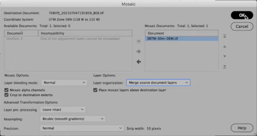
I’ve grabbed a 30m SRTM DEM for this area. I can use this as a mask to get rid of those pesky mountain shadows. The tricky part is that we are now working with mixed projections and different datasets.

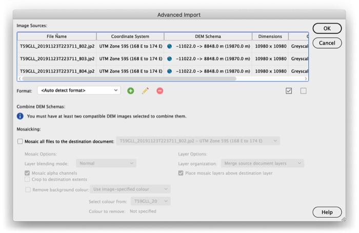
I can use the nifty Mosaic tool in Geographic Imager to bring these two datasets together. The really important part is to specify the “crop to destination extents” option. Doing this will not only apply an on-the-fly projection transformation but also crop the large DEM dataset automatically down to match my water mask layer. Also, be sure to select the “merge source document layers” option – this really helps clean up the layer management, while still keeping the important stuff separate.

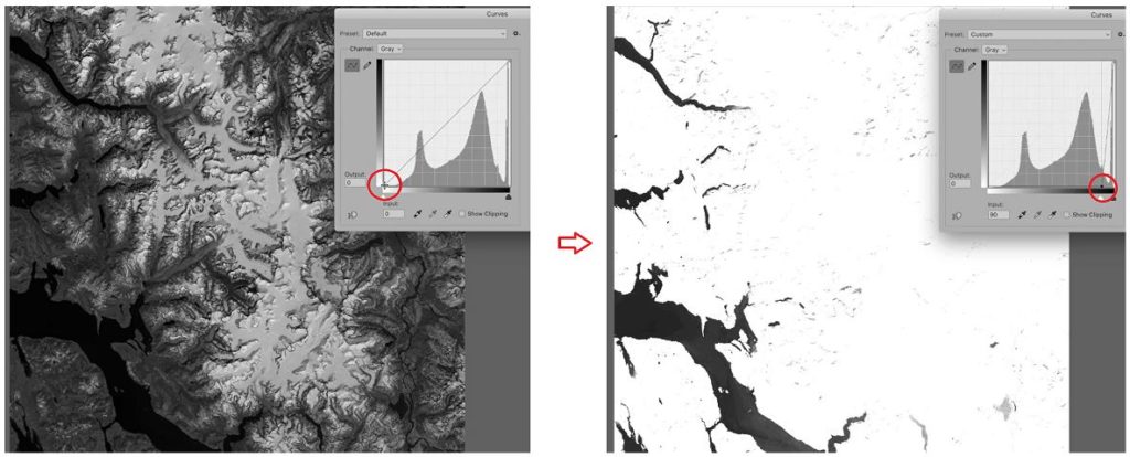
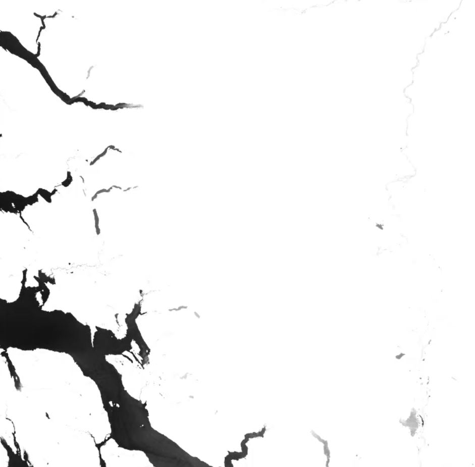
To get rid of those mountain shadows, we apply another linear curves adjustment. Similar to before, the idea is to compress that tonal range until only the regions at or near sea level are visible (most of the water in our image is at sea level).

Select the layer, apply the “Screen” blending mode, and then “flatten” the image to create the final water mask layer (now with removed mountain shadows!).

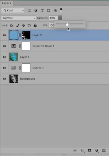
Apply the Water-mask layer

When the water mask is ready, copy it to the computer clipboard. Next, go back to the true color image and create a new topmost layer and add a layer mask. Then paste this into the layer mask (be sure to invert it!). You can then fill the water layer with whichever flat blue that you like. Finally, partially decrease the opacity of the flat blue layer to reveal any sediments or reflections that may exist in the satellite images. You might need to do a bit of manual touch-up with the brush tool on your mask layer to completely remove all mountain shadows.

Mosaic Multiple Images

I did almost the exact same technique on another image directly south of this one, and I’ve decided I would like to mosaic both of these images together into a single composite. Again, I use the mosaic tool (this time uncheck the “crop” option), and voila! Both images are mosaiced together in less than a second!
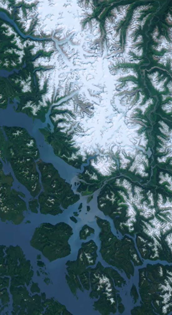
Finishing Touches

A few more touch-ups with the gradient tool to blend the images at their border, and some final adjustment layers to boost the saturation a bit and we are basically done.

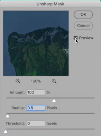
The very last thing that I do is to apply sharpening, which is irreversible. You will need to experiment to determine the amount that is best. As a starting point, try these settings (Filter/Sharpen/Unsharp Mask). Amount = 100%, Radius = 0.5 pixels, Threshold = 0 levels

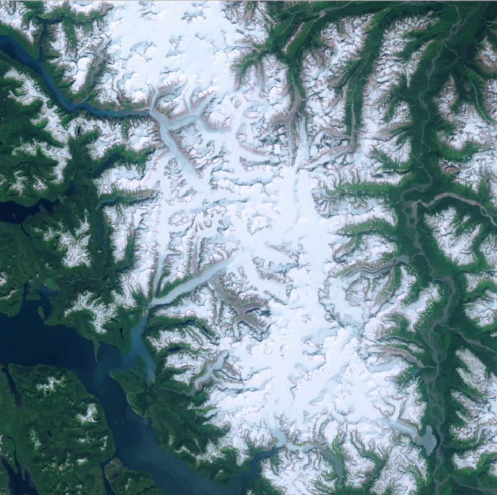
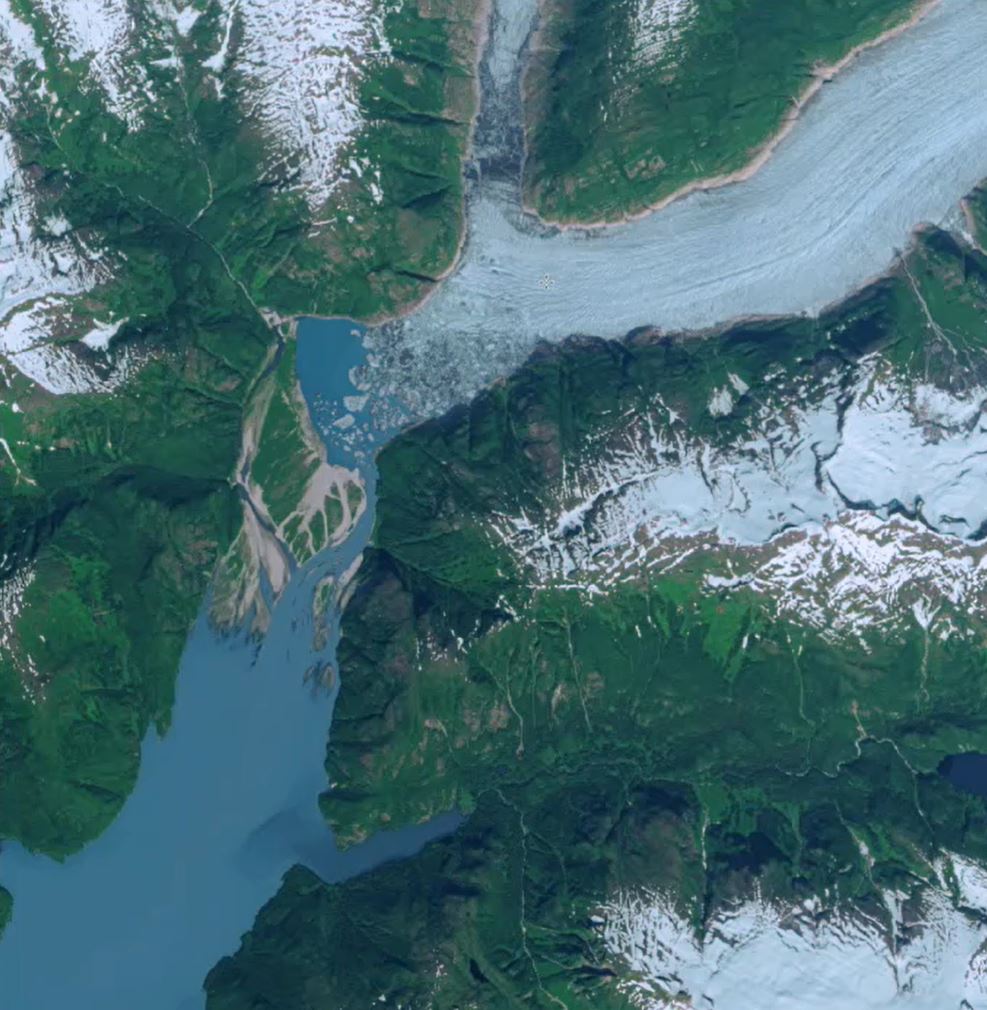
That’s it! We took some really nice multispectral Sentinel-2 Imagery, some great tools in Geographic Imager, and used some of the nice native Photoshop tools to create a really vibrant, true-color image that’s ready to be draped over some 3D relief or used to create another nice map!

A note on Exporting Images

Before exporting the final image as a GeoTIFF using Geographic Imager, go to Image/Mode and reduce the bit depth from 16 to 8 bits per channel, and then flatten the image. This will significantly reduce the file size.

***

About the Author

Tom Patterson worked as a cartographer at the U.S. National Park Service, Harpers Ferry Center until retiring in 2018. He has an M.A. in Geography from the University of Hawai‘i at Mānoa. Presenting terrain on maps is Tom’s passion. He publishes his work on shadedrelief.com and is the co-developer of the Natural Earth dataset and the Equal Earth projection. Tom has served as President and Executive Director of the NACIS. He is now Vice-Chair of the International Cartographic Association, Commission on Mountain Cartography.

Mapping Class: Work with Sentinel-2 Imagery in Geographic Imager – Part One, with Tom Patterson

Welcome to the latest edition of Mapping Class! The Mapping Class tutorial series curates demonstrations and workflows created by professional cartographers and expert Avenza software users. In this month’s edition, we welcome Tom Patterson, a map-maker extraordinaire and a true household name in the cartography world. Today Tom is sharing with us a demonstration showing how he works with Sentinel-2 Imagery Data using Geographic Imager and Adobe Photoshop. Tom uses a new dataset that that represents a “pretty difficult” image to process and offers an excellent look at how to create beautiful natural colour images from satellite data.

Part One of this exciting walkthrough covers the techniques Tom uses for accessing and importing satellite imagery data, as well as his approach to colour correction using some of the powerful built-in image editing tools in Adobe Photoshop. Tom has produced video notes below to help you follow along! Look out for Part Two, coming in next months edition of Mapping Class!

***

Work with Sentinel-2 Imagery in Geographic Imager: Part One
by Tom Patterson (Video notes adapted from original)

This tutorial explains how to process Sentinel-2 satellite data, released by the European Space Agency for free, into natural colour images. Beautification is the goal—nature often can use a little help when using satellite images for maps and graphical presentations.

To do this tutorial you will need Adobe Photoshop and Avenza Geographic Imager. Trial versions for geographic imager can be found here. For this tutorial, you should also have intermediate Photoshop skills, a good internet connection, and a computer with plenty of RAM.

Getting the data

The US Geological Survey distributes Sentinel-2 data on the EarthExplorer data portal. You can also download Sentinel-2 on the Copernicus Open Access Hub, although I find EarthExplorer easier to use.

1) Downloading data from EarthExplorer requires that you first sign in as a registered user.

2) After you sign in, use the “Search Criteria” tab in the upper left to specify a point of interest. You can also draw a polygon on the map to specify a larger search area.

3) Click the “Data Sets” tab next. From the long list of data types, select “Sentinel-2.”

4) The EarthExplorer portal offers useful tools for narrowing your search. For example, you can filter by acquisition date and cloud cover. Sentinel-2 image extents are viewable as transparent map overlays. 

5) Click the “Results” tab to peruse the available images. Then click the image thumbnails to see larger image previews in false color. Scrolling down from the image previews reveals additional metadata

To download a scene from the search results list, click the “Download Options” icon. You will then see these two download options:

● L1C Tile in JPEG2000 format (XX MB)

● Full Resolution Browse in GeoTIFF format (XX MB)

Download both.

7) The Full Resolution Browse in GeoTIFF format is a false-color image (bands 11, 8A, and 4) at 20-meter resolution.

8) Decompress the L1C Tile in JPEG2000 format archive. It contains the raw Sentinel-2 bands and a true-color image. You will need to drill through multiple folders to get to these data 

Importing the data

Because Photoshop does not natively import JPEG2000 files, you will need to use a Geographic Imager to import the Sentinel-2 data. The advantage of Geographic Imager over other plugins is that it preserves georeferencing and allows you to export manipulated Sentinel-2 images as GeoTIFFs.

1) In the Photoshop drop menu, go to File/Import/GI: Advanced Import

2) Select one or more Sentinel-2 bands to import (in this case, we want Bands 4, 3, and 2 which correspond to our Red, Green, and Blue bands) and click OK. Importing could take a minute or two to complete. Each Sentinel-2 band will open as a separate Photoshop file. That’s it.

Colour Correction

The premade True Color Images are convenient to obtain, and you can easily adjust them to create acceptable results. However, they have an Achilles heel: snow- and ice-covered landscapes. Automated processing removes the very lightest tones, rendering them as empty white (below, left). In order to depict subtle details in snowy terrain, one must build the satellite image from scratch using the raw data in bands 4, 3, and 2 (below, right).

1) Use Geographic Imager to open bands 4, 3, and 2 (File/Import/GI: Advanced Import…). The import will take a couple of minutes to complete, and the three bands will open as separate Photoshop files.

2) With one of the Photoshop files active, go to the flyout menu in the upper right corner of the Channels window. Select Merge Channels…

3) In the Merge Channels window, change the mode to RGB Color and specify 3 channels.

4) Another window will pop up. Make sure that band 4 is the red channel, band 3 is the green channel, and band 2 is the blue channel. Then click okay.

5) Photoshop will then ask whether you want to save each of the three bands. Don’t save them. You will then see the merged 16-bit RGB image, which is mostly gray

Using Curves

Now the fun begins. Compared to Levels adjustments that are linear, Curves adjustments are non-linear, giving you more control over discrete portions of the tonal range in an image. They are a little tricky to use at first, but the precise results that you can achieve with this command make learning it very worthwhile.

1) Apply a Curves adjustment layer and adjust the tonal range of the image taking care to leave some value in the snow patches. I often apply two or more Curves adjustment layers, one on top of the other, to fine-tune the tonal balance. With 16-bit images, you can stretch the tonal range without worrying about banding artifacts.

2) Save your applied curves as adjustment layers so you can save and re-use them for later. This is especially important when you start mosaicing imagery data (coming in part two!) and need to ensure curves are applied consistently across multiple images.

Below is the curve that I used to adjust the image. The histogram shows the distribution of light and dark values. Moving the lower-left end of the curve to the right lightened dark trees. Moving the top-right end down added a slight amount of tone to the white snow. Both of these moves decreased overall contrast.

Touch-up with the False Colour Image

We want to add a bit more eye-catching vibrance to our image. We can do that by utilizing the included false colour imagery and using the colour properties and blending tools to really make the mountainous terrain pop. 

1) Since we need the false colour imagery to match the resolution of our RGB image, we need to upscale it. This can be done using the image sizing properties and resampling using the “Preserve Details” setting.

2) Overlay this upscaled false colour image over top of the RGB layer. You can then adjust the blending modes to create a nice vibrant image. In this case, I use the “Soft Light” blending mode, which is great for making the alpine terrain really stand out.

3) Create a selective colour adjustment layer to touch out individual colour tones in the image. For example, I try to remove much of the yellow tones in the image, as yellow tones are atypical for the “cold” alpine-like terrain we find in this image. 

Coming up in Part Two:

The land areas in this image now stand out quite well. They look quite a bit more vibrant than the raw data and offer a bit better tonality than what we find in the automatically generated true-colour image included in the download. What we can do next is work on making the water areas stand out as well. I’ll show you how you can use the mosaic tool in Geographic Imager to work with elevation data to create layer masks that make adjusting water areas easy.

***

About the Author

Tom Patterson worked as a cartographer at the U.S. National Park Service, Harpers Ferry Center until retiring in 2018. He has an M.A. in Geography from the University of Hawai‘i at Mānoa. Presenting terrain on maps is Tom’s passion. He publishes his work on ShadedRelief.com and is the co-developer of the Natural Earth dataset and the Equal Earth projection. Tom has served as President and Executive Director of the NACIS. He is now Vice-Chair of the International Cartographic Association, Commission on Mountain Cartography.