My Account     Contact Us     Cart

Exploring Shaded Relief Techniques in Geographic Imager and Adobe Photoshop 3D

PLEASE NOTE: As of Photoshop 22.5, Adobe has discontinued support for the program’s 3D features. This may affect some or all elements of this blog. For more information, see Adobe’s FAQ page about this change and the Geographic Imager compatibility information page.

In the world of map-making, shaded relief refers to a visual technique that gives the illusion of three-dimensional terrain on an otherwise flat map. Cartographers use shaded relief to draw the viewer’s eye to prominent topographic features such as mountains, valleys and canyons. Using imaginary illumination sources and digital elevation data to cast directional light on a map, the cartographer can give the illusion of depth, casting shadows into valleys and lowlands, and highlighting ridgelines and peaks as if they are bathed in sunlight. 

Historically, this technique was achieved entirely by hand and was extremely labour intensive. Now, with modern graphical software and digital mapping technologies, relief shading can be accomplished right on the desktop. 

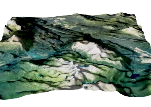
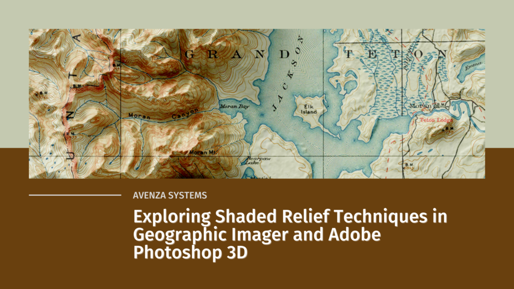
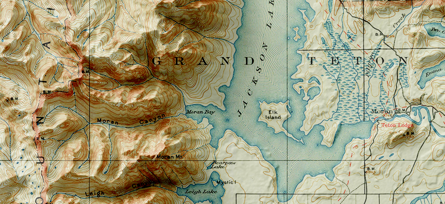
To demonstrate this, we are going to use the powerful spatial imagery tools and graphical design capabilities of the Geographic Imager plug-in for Adobe Photoshop to explore relief shading using a really interesting 19th-century historical map. Here is a sneak peek to show what the final product will look like.

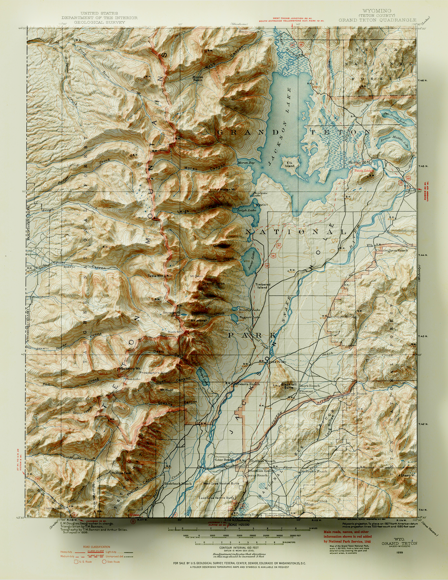
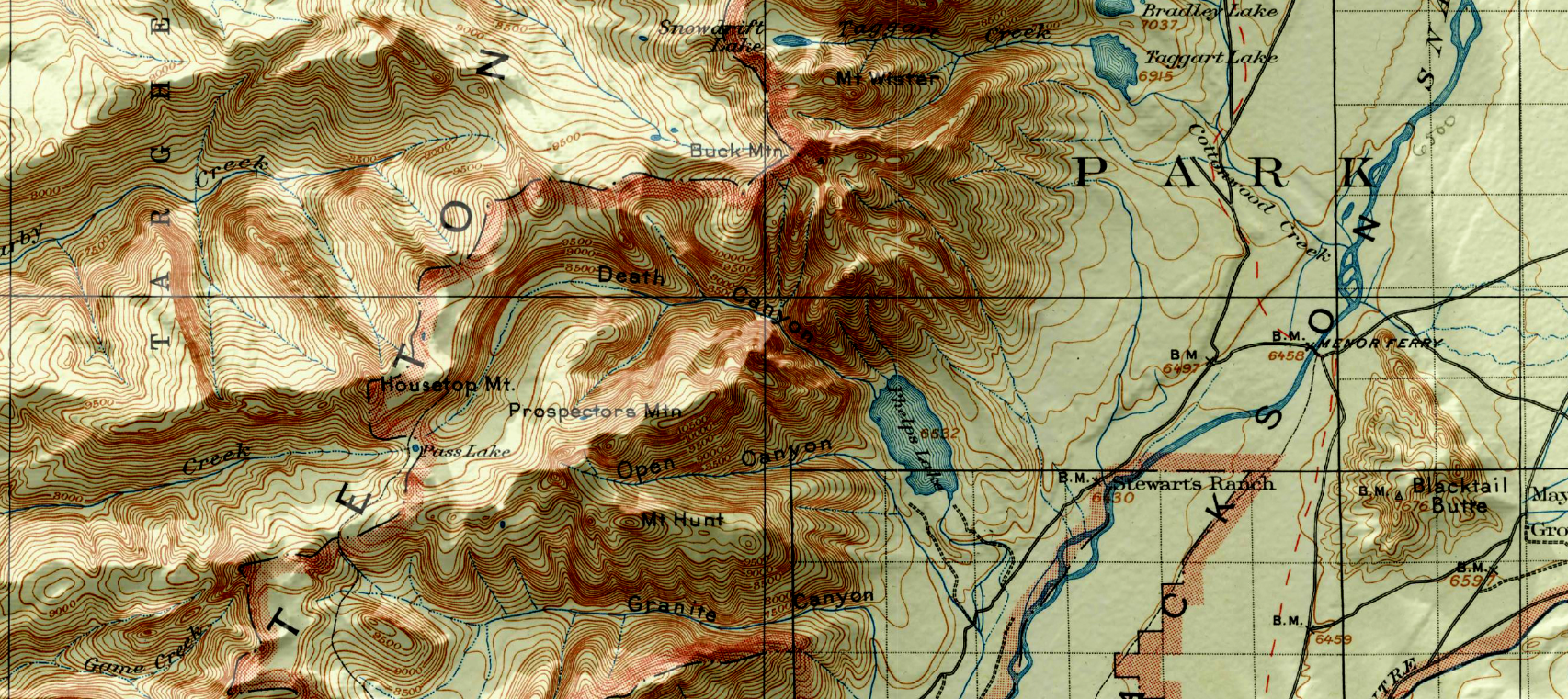
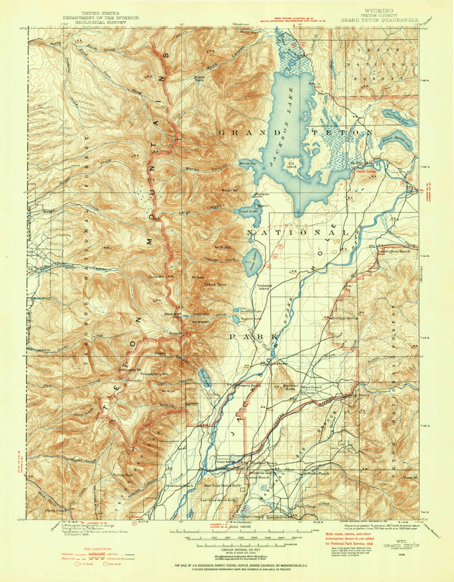
Let’s start with our original map. We have taken an absolutely stunning United States Geological Survey Map of the world-renowned Grand Teton National Park in Wyoming. Originally drafted by hand in the year 1899, the map features beautifully drawn contour lines and colour work showing the mountainous topography of the park and its surrounding area. The map, and thousands of others like it, are available in full-resolution on the USGS Historical Map Catalogue. Our goal will be to bring the map to life using three-dimensional (3D) relief shading techniques available with Geographic Imager and Adobe Photoshop.

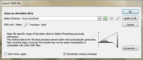
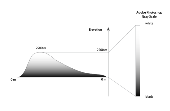
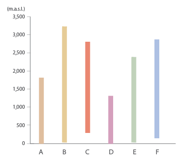
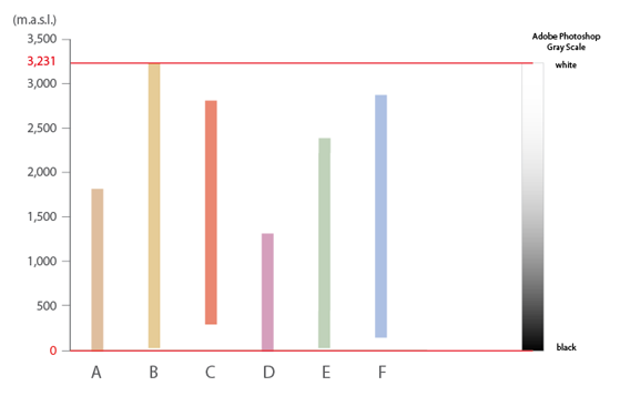
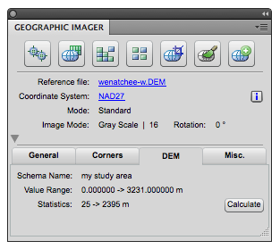
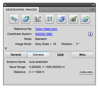
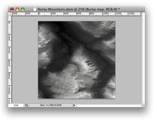
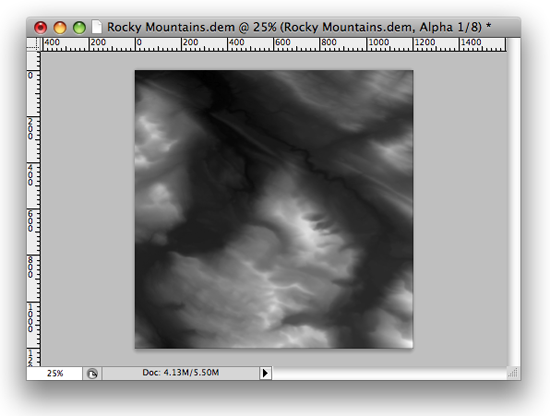
First, we need to bring in some elevation data. Elevation data is critical for creating shaded relief, as it determines how light and shadows will behave in different parts of the map. We can obtain high-resolution digital elevation models (DEM) for our region from the USGS EarthExplorer.

Those of your familiar with spatial imagery data and DEMs will know that our first challenge will be working with tiled (discontinuous) imagery data products. In its raw form, DEMs are often stored as identically sized tiles, with each tile representing a specific indexed region of the earth’s surface. It is an unfortunate reality that many times the spatial extent of each DEM tile rarely matches the exact extent of the area you are interested in mapping. As a result, map-makers and spatial imagery specialists need to implement tools to import, merge, and crop these tiles to a more useful format and size.

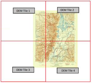
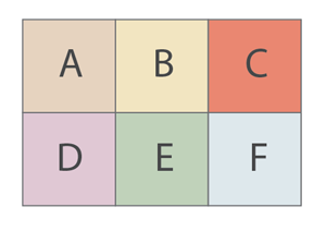
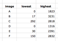
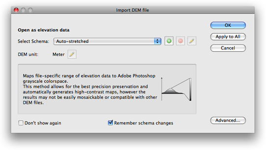
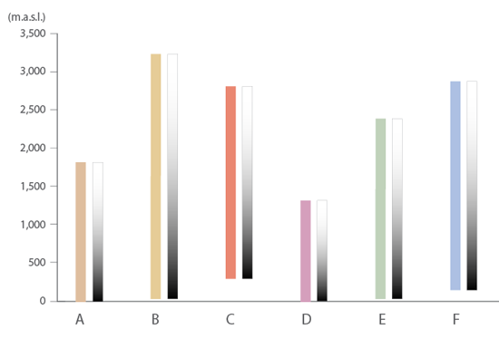
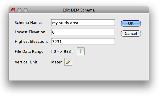
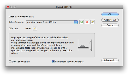
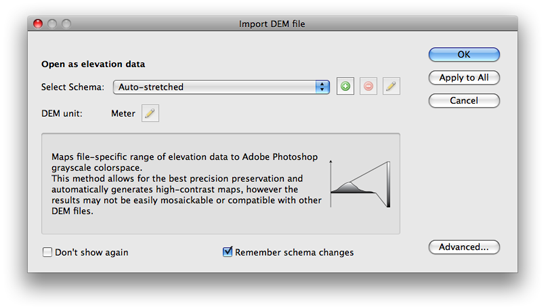
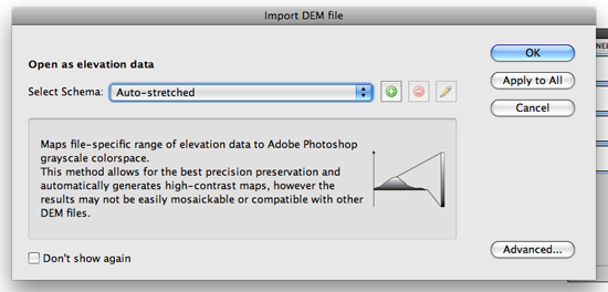
In our case, the elevation data for the area shown by the original 1899 topo-map is now represented by four separate DEM tiles, with roughly one tile for each quadrant of the map. To handle this problem, we can use the powerful Advanced Import tool within the Geographic Imager toolbar. The tool is a one-stop solution to easily import and mosaic our DEM datasets directly into Photoshop, all while retaining the spatial awareness we need to georeference or transform our data layers.

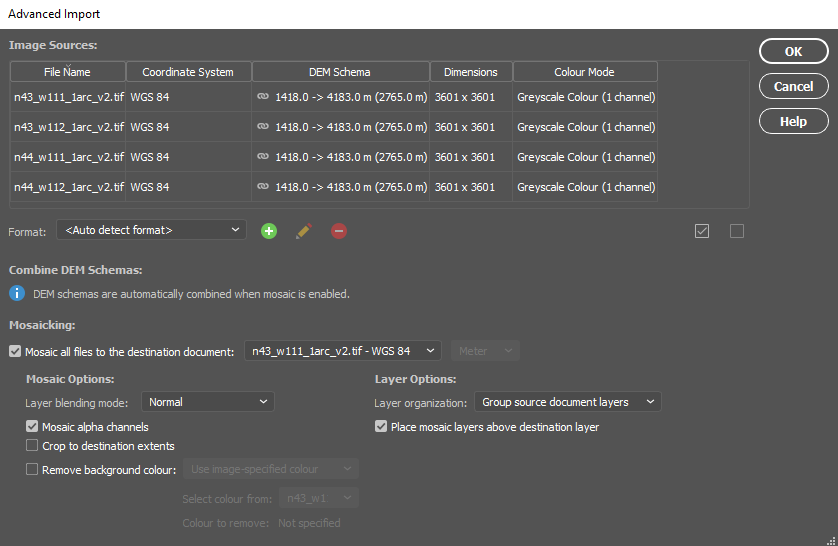
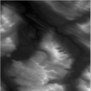
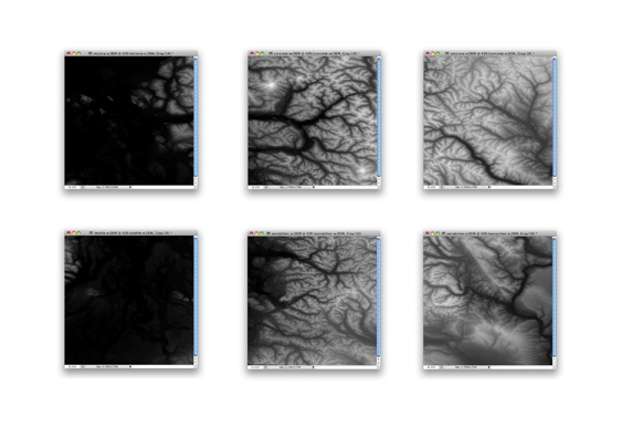
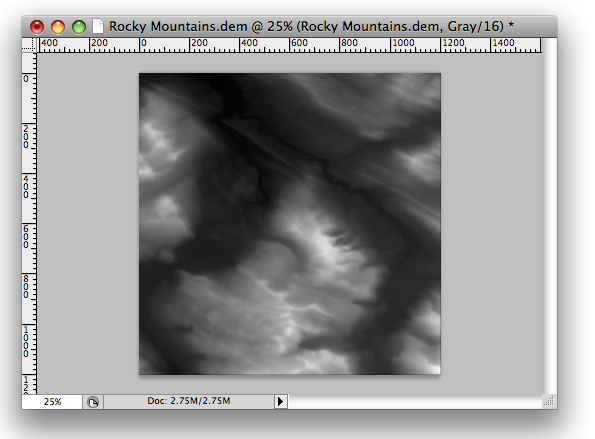
By combining each of the four raw DEM datasets, the tool will mosaic the tiles into a single merged, continuous, and geographically accurate elevation layer covering the entire extent of the map. Even more impressive is that Geographic Imager can use the spatial referencing information in the data to automatically align and overlay the original 1899 topo map onto the elevation layer, removing the need to perform manual georeferencing. (If the imagery data you are using does not have spatial referencing information already, don’t worry – our support team has crafted some excellent, easy to follow georeferencing in Geographic Imager tutorials).

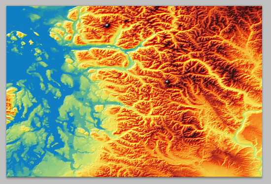
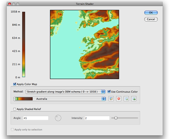
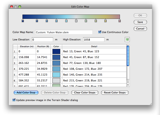
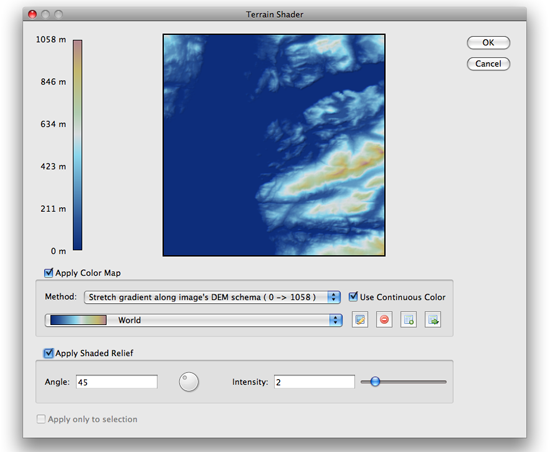
With our DEM data imported into Photoshop, we can start to explore different techniques for creating shaded relief. We will start by using the Terrain Shader tool located on the Geographic Imager toolbar. Terrain shader is a one-click technique to create simple shaded relief instantly. It allows you to configure the angle and intensity of the simulated illumination source to control the prominence and direction of casted shadows. Additionally, you can apply customized colour gradients to easily produce stylized elevation maps or apply hypsometric tints. 

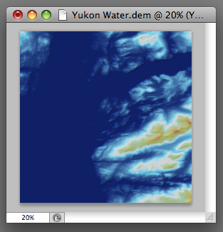
In many situations, the Terrain Shader tool is an all-in-one, quick and easy way to create shaded relief. The output of the tool makes it easy to distinguish topographic features and can be used to quickly produce a shaded-relief backdrop for your map.

One of the greatest benefits of using Geographic Imager is that we retain all the imagery manipulation and spatial referencing capabilities of a GIS while still having access to the massive inventory of powerful image editing tools provided by Photoshop. This allows us to take our shaded relief technique up a notch by incorporating the advanced 3D rendering and lighting tools of Photoshop 3D to truly bring our 1899 Grand Teton survey map to life.

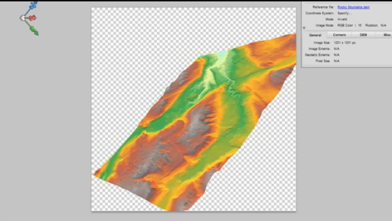
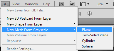
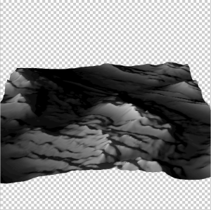
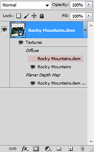
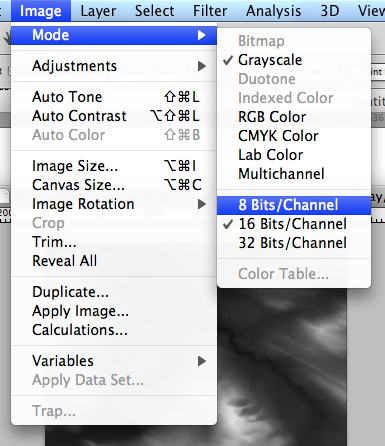
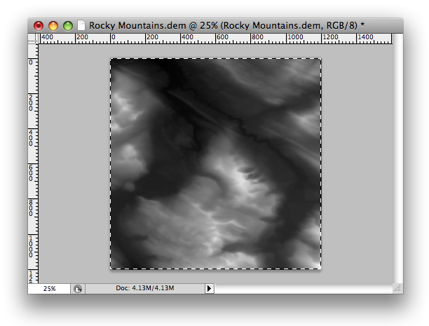
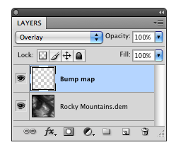
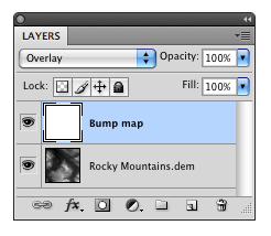
To start, we first need to trim the DEM layer down to our specific area of interest. We used the GeoCrop tool to crop our mosaiced DEM layer down to the exact extent of our topo map (it is important that both layers are the exact same extent – you’ll see why later). Next, we can open up the Photoshop 3D toolbar, and convert our flat DEM into an extruded 3D “Depth Map”. 

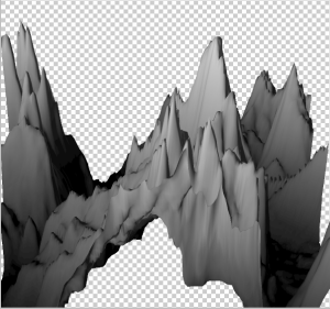
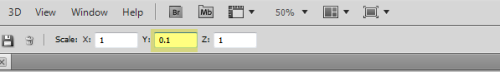
To enhance the shaded relief effect, we need to apply a vertical exaggeration to the model. In 3D mode, we can drag the z-axis scaling slider to exaggerate the prominence of the topographical features in our map. By creating vertical exaggeration, we can create more pronounced shaded relief, as canyons and lowlands will capture shadows more effectively.

In 3D mode, we can use the mouse cursor to pan and rotate our “camera” to get different perspectives of our elevation model. This can be useful for creating orthographic or oblique perspective map styles.

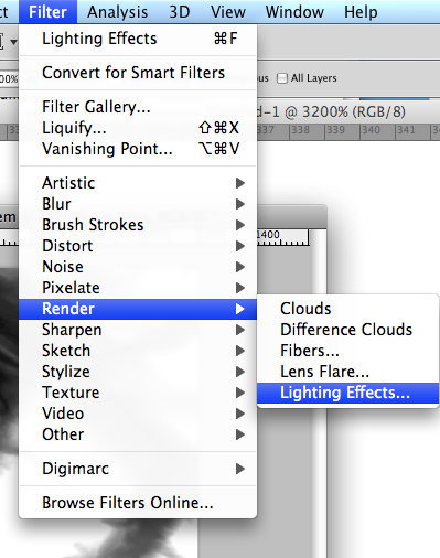
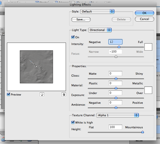
Now that we have a configured 3D model of our map area, we can apply our simulated illumination source. Much like the Terrain Shader tool, we can control the illumination intensity and angle of approach. Since we are working in a 3D environment however, we now have three different axes that control where our light is coming from. Notice how the angle is important for affecting the length and intensity of shadows in our relief map. This includes the prominent mountain silhouettes that can be created when we set the light source to approach from a low angle on the horizon.

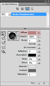
Next, we can configure the surface properties and apply a texture overlay to our 3D model. Experimenting with these settings changes how light interacts with the surface and can be refined to produce different relief shading effects. Using these surface properties, we can also drape the original 1899 Topo map onto our surface model (this is why it is important for both the DEM and the topo-map to share the exact same extent, otherwise the topo map will be distorted once it is draped over the surface).

Fine-tuning the map at this stage can take some time and experimentation. We can add some additional light sources with different casting angles and intensity to help create a multi-directional hillshade effect. We can also configure the light settings to produce softer, less pronounced shadows that look more realistic. After spending some time adjusting the lighting and surface settings, as well as configuring the camera view angle,  we can hit the “render” button and sit back while it creates a full-resolution rendering of our 3D model (this part can be very computationally intensive, and may require a high-performance machine to process efficiently).

Since we are still creating our map entirely within the Photoshop environment, we can immediately fine-tune the brightness, contrast, and colour of our map before exporting the final product. 

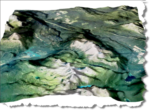
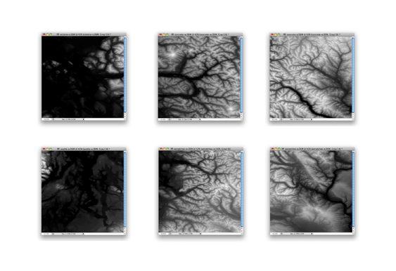
You can see some renders of the final map below. Thanks to the powerful spatial import and manipulation tools of Geographic Imager, and the ability to work entirely within the advanced image editing environment of Photoshop, we were able to create a dramatic 3D shaded relief effect that brings our 1899 USGS Grand Teton Survey map to life.

3D Terrain Model using Geographic Imager

PLEASE NOTE: As of Photoshop 22.5, Adobe has discontinued support for the program’s 3D features. This may affect some or all elements of this blog. For more information, see Adobe’s FAQ page about this change and the Geographic Imager compatibility information page.

We created a video to show that it is possible to use geospatial data and the 3D capabilities of Adobe Photoshop. It performs very well with a decent computer and video card.

In this video, a combination of Geographic Imager and Adobe Photoshop functions are used to open a DEM file using a script. The script also transforms a DEM into a 3D model and allows for an overlay of a colour model based on the data or a custom image (e.g. ortho image). Video after the jump.

How to Create a 3D Rendition of a DEM With a Draped Image

PLEASE NOTE: As of Photoshop 22.5, Adobe has discontinued support for the program’s 3D features. This may affect some or all elements of this blog. For more information, see Adobe’s FAQ page about this change and the Geographic Imager compatibility information page.

NOTE: Prior to performing these steps with your data you would want to ensure that the DEM and image have the same geographic extents.

Item 2: Coordinate system of the map

Using Geographic Imager, open your DEM file and set the desired schema type. In this case the DEM was “Auto stretched”.

Item 2: Coordinate system of the map

With the DEM now opened and rendered as a 16-bit grayscale Image we can now make use of a number of Adobe Photshop tools to render it in 3D and to drape the image.

Item 2: Coordinate system of the map

The following steps will outline the Adobe Photoshop procedures required to create the 3D rendition:

1. Create a 3D mesh: Under the 3D menu within Photoshop select “New Mesh From Grayscle->Plane”

Item 2: Coordinate system of the map

2. We then use the “3D Object Rotate Tool” located in the Photoshop toolbar to manually rotate the mesh tilting it backwards, resulting in something like this

Item 2: Coordinate system of the map

3. The resulting mesh is too exaggerated for a realistic rendering of the landscape so we will adjust the y orientation of it using the “3D Object Scale tool” setting the Y: scale to 0.10

Item 2: Coordinate system of the map

This is the image after vertically rescaling it

Item 2: Coordinate system of the map

4.Once the 3D mesh has been rescaled the image can be draped

In the Adobe Photoshop “3D Materials” panel, click the “Edit Diffuse texture” button (as denoted in the screenshot below) and select the “Load Texture” option. Now locate and select the image you wish to drape on the 3D mesh.

Item 2: Coordinate system of the map

5. Within the Layers panel turn off the visibility of the Rocky Mountain DEM (as in the screenshot below).

Item 2: Coordinate system of the map

The end result should be a 3D model such as this.

Item 2: Coordinate system of the map

Geographic Imager 3.2: Introduction to Terrain Shader, Part 3 – Applying Terrain Shader to multiple DEM files

If your workflow involves Terrain Shader, specifying a DEM schema is an important step, especially when dealing with mulitple DEM files.

When importing a single DEM file, Geographic Imager converts elevation values to gray scale values. For example, if the elevation range in your DEM file is between 0 and 2500 meters and the “Auto-stretched” option is selected, this range will be converted to the Adobe Photoshop gray scale range between black and white. As shown below, the black color is assigned to the lowest elevation value (0 meter) while the white color is assigned to the highest elevation value (2500 meters). For elevation values between 0 and 2500, Geographic Imager calculates and converts them into gray scale.

Import DEM File - Auto-stretched

In this example, we’ll use six DEM files of one geographic region. Many datasets are distributed as tiled DEM files. Each of them is next to each other and the goal is to create a colorized DEM image from those six files.

Collected 6 dem files

When dealing with multiple DEM files, you will need to consider the elevation range of the each DEM file. In other words, the elevation range in each DEM file will be slightly different.

table: elevation range in each DEM file Chart: Elevation range in each DEM files

Option 1: Using the “Auto-Stretched” option for multiple DEM files

When importing multiple DEM images and using the “Auto-stretched” option, click “Apply to All”…

Dialog window: Import DEM file - auto stretched

Every one of the DEM images will be converted to the gray scale between black and white.

graph: stretching the gray scale to every image file

As a result, you can get the maximum contrast in each image. However, you will not be able to mosaic or apply Terrain Shader to those six images because each DEM has slight differences in elevation and an all encompassing schema like the”Auto-stretched” option will not work.

DEM images opened with Auto-stretched

Option 2: Creating a DEM schema by specifying a range

In order to apply Terrain Shader to multiple DEM files, you will need to assign one DEM schema to each DEM image you would like to share the same schema.

Step 1: Identify the elevation range amongst multiple DEM files

Explore the DEM files and find out what the elevation range is for each one. Then note which are the lowest and highest values among all DEMs. For this example, the lowest elevation is 0 m and the highest is 3,231 meters.

Finding the range among multiple DEM files

Step 2: Create a new DEM schema for your dataset

Choose File > Open and select multiple DEM files. Once the Import DEM file dialog box is open, click the Add button to open the “Edit DEM Schema” dialog box.

Create a new Schema name (e.g. “my study area”). Simply enter the lowest and highest elevation value found in Step 1.

Dialog window: Edit DEM Schema - specifying the range for the DEM schema

Step 3: Apply the DEM schema to your datasets

When you’ve created a new DEM schema, it will be available in the “Select Schema” drop-down list. Choose the new schema and click “Apply to All”. This selected schema will be applied to all the DEM files being imported.

dialog window: Importing DEM file with the same schema

After the import process is completed, the images are ready for Terrain Shader.

All the DEM files imported with the same DEM schema

When one of the imported DEM file is the active document, click the “DEM” tab in the Geographic Imager panel. It shows the DEM schema name, the DEM value range, and the actual elevation value available in the currently active document. Click the “Calculate” button if you do not see the statistics (actual elevation value range of the active document).

Geographic Imager Main Panel

Step 4: Apply Terrain Shader to your DEM files

Since each DEM has a schema, a mosaic can be perfomed and then Terrain Shader can be applied to the mosaicked iamge.

DEM files mosaicked and Terrain Shader effect is applied

Geographic Imager 3.2: Introduction to Terrain Shader, Part 1

The upcoming release of Geographic Imager 3.2 introduces a new feature called Terrain Shader, used to apply color gradients and shaded relief to imported DEM images. Color gradients can be exported so that you can use them for other images or share them with other people.

You might want to take a look at our brief video about the Geographic Imager Terrain Shader on our Avenza YouTube channel.

In this blog, I’ll show you a quick workflow with Terrain Shader using one of the files from the Geographic Imager tutorial folder.

1) Open the DEM file called Yukon Water.dem from the Geographic Imager Tutorial Folder in Adobe Photoshop. Geographic Imager will automatically detect the file type so that you will see the “Import DEM File” dialog box(below).

When your workflow involves Terrain Shader, it is important to select an appropriate schema in the Import DEM file dialog box. For now, we’ll use the option “Auto-stretched”. We’ll return to this dialog box when we talk about an advanced use of Terrain Shader feature in another blog.

Importing a DEM file

After the DEM file is successfully imported, you will see the geospatial information, the DEM schema and the value range information in the Geographic Imager panel. The panel has been redesigned and improved for version 3.2 (We think it works really well!)

Geographic Imager Main Panel: displaying the information of the dem file just imported

2) Click the Terrain Shader button.

Terrain Shader icon on Geographic Imager Main Panel

In the Terrain Shader dialog box, on the left side, you can see the elevation range of the DEM file. There is a large preview image at the centre of the dialog box.

Terrain Shader Main Dialog Window

3) Click the check box beside “Apply Color Map” to apply a color gradient to the DEM image.

You can select one gradient from the preset gradients from the dropdown menu. Or you can edit the color gradient form the existing one. Click the pencil icon next to the preset dropdown menu. In the Edit Color Map dialog box, you can modify the gradient scheme. You can change colors, add ramps, adjust the ramp position, ….etc.

Editing Color Scheme

4) Click OK to apply the modication.

5) Another great function with the Terrain Shader is to apply the shaded relief effect at the same time. Click the check box beside “Applly Shaded Relief”.

You can adjust the angle of the source light and the intensity of the contrast. You can see how the settings affect the DEM image in the preview.

Applying a shaded relief effect

6) The DEM is stylized with a color gradient and a shaded relief effect.

colorized dem image with a shaded relief effect

Stay tuned for Introduction to Terrain Shader, Part 2

Geographic Imager: Create shaded relief from a DEM

With Geographic Imager 3.x, you can import DEM files to Adobe Photoshop and can create shaded relief images.

step 12: Shaded relief image completed

There are two methods to achieve this:

Method 1: Run the pre-made JavaScript and apply it to all images

After opening your DEM image, choose File > Scripts > Browse… and select Shaded Relief.jsx from the SampleScripts folder inside the Geographic Imager Tutorial folder. It will generate the shaded relief image for the opened DEM image based on the settings in the JavaScript file.


Method 2: Create shaded relief images manually

We’ll use the DEM file Rocky Mountains.dem available in the Geographic Imager Tutorial folder for this demonstration.

1) Open the Rocky Mountains.dem image from the Geographic Imager tutorial folder. Geographic Imager automatically detects it as a DEM file and provides the option to select the DEM image import method. For this demonstration, choose Auto-Stretched from the Select Schema drop-down list.

Step 1: Import DEM file option

The imported DEM is opened in black and white. Take a look at the header of the image (or tab of the image file). Notice that it displays “Gray/16”. This indicates that the image is in the 16 Bits/Channel Grayscale mode.

step 1: Imported DEM image

2) Now, change the image mode from 16 Bits/Channel Grayscale to 8 Bits/Channel RGB. From the top menu bar, choose Image > Mode and then 8 Bits/Channel. Once again, go to Image > Mode, this time choose RGB Color.

step 2: Changing the color mode

Once completed, take a look at the image header again (or file tab). Now “RGB/8” is indicated in the header, meaning that the image is now in the 8 Bits/Channel RGB color mode.

step 2: Color mode changed

3) Select the entire canvas (use the Rectangular Marquee Tool) and copy the selected area to the clipboard (Edit > Copy).

step 3: Select the entire canvas

4) Open the Channels panel (Window > Channels) and add one Alpha channel by clicking the Create new channel button at the bottom of the panel or go to the panel option menu and choose New Channel. Leave the channel name as “Alpha 1”.

step 4: create a new channel

5) Select the “Alpha 1” in the Channels panel and fill it in white using the Paint Bucket Tool.

step 5: Filling Alpha channel

6) In step 3 we copied the selected area (the entire canvas) to the clipboard, now we’re going to paste it to the new channel. Select “Alpha 1” in the Channels panel, and paste it (Edit > Paste). You can see that the same image is displayed for all the channels when the copied area is successfully pasted. Make the Alpha 1 channel invisible and make sure the RGB channels are visible.

step 6: pasted canvas

7) Deselect the area (Select > Deselect from the top menu bar).

step 7: deselected area

8) In the Layers panel (Window > Layers), create a new layer named Bump map. Change the Blending mode to Overlay. step 8: New Layer "Bump map"

9) Using the Paint Bucket Tool again, fill the new “Bump map” layer with white.

step 9: fill white

10) From the menu bar, choose Filter > Render > Lighting Effects…

step 10: Menu Filter > REnder > Lighting Effects ...

11) Adjust the settings in the Lighting Effects dialog window.

step 11: adjusting the light effect

12) The shaded relief image is completed! You can use this image to overlay with other georeferenced images with Geographic Imager or with vector datasets with MAPublisher.

step 12: Shaded relief image completed