In a previous blog post, we defined a few common cartography terms that you might be likely to encounter while using MAPublisher and Geographic Imager; however, that was just the tip of the iceberg when it comes to cartography and GIS jargon. Here, in no particular order, are several additional terms used by cartographers, GIS professionals and people who work with spatial imagery.
Topology
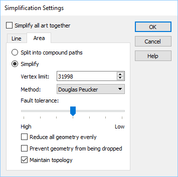
Topology is a key principle in GIS for data management and integrity, ensuring the data quality of spatial relationships is maintained. In general, a topological data model defines how spatial objects (point, line, and area features) are represented, and defines and enforces data integrity rules (for example, there should be no gaps between polygons).
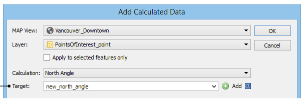
Azimuth
The horizontal angle, measured in degrees, between a baseline drawn from a center point and another line drawn from the same point. Normally, the baseline points true north and the angle is measured clockwise from the baseline.
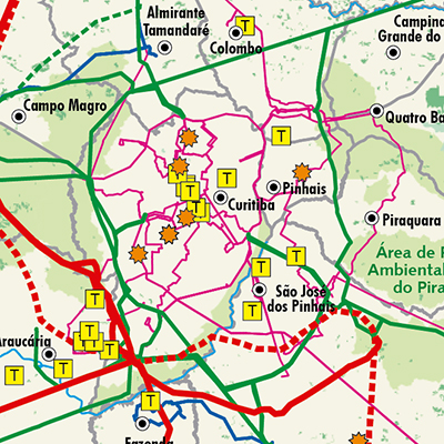
Neatline
All 2-dimensionally rendered maps have to compromise somewhat on accuracy, even if only just a little by moving or scaling features to improve readability. However, the neatline is never adjusted, making it the most accurate element on a map.
The neatline is the border defining the extent of geographic data on a map and separating the body of the map from the map margin. It demarcates map units such as meridians and parallels, and depending on the map projection and the units selected, the neatline may not have 90-degree corners.
Geodatabase
A Geodatabase, a database or file structure used primarily to store, query, and manipulate spatial data, stores geometry, a spatial reference system, attributes, and behavioral rules for data. An advantage of geodatabases over shapefiles is that various types of geographic datasets can be collected within a geodatabase, including feature classes, attribute tables, raster datasets, network datasets, topologies, and many others.
Geoprocessing
Geoprocessing is an operation used to manipulate a GIS data resulting in a new set of data. Common geoprocessing operations include geographic feature overlay, feature selection and analysis, topology processing, raster processing, and data conversion. Geoprocessing allows for the definition, management, and analysis of information used to make decisions based on patterns within the GIS data.
Shapefile
An Esri Shapefile is a vector data storage format for storing the location, shape, and attributes of geographic features. A shapefile is stored as a set of related files and contains one feature class. An alternative to using shapefiles to store GIS data is a geodatabase, however, shapefiles have some advantages in terms of relative simplicity and wide-ranging compatibility with many applications. Related files contain additional information that is read by the shapefile when opening/importing in GIS applications, as long as these related files have the same name and reside in the same directory – the *.dbf (database) file contains attribute information, and the *.prj (projection) file contains coordinate system information. Shapefiles also have limitations such as the inability to support raster files, and large file sizes.
Buffer
A zone around a map feature measured in units of distance or time is called a buffer. Buffers are useful for proximity analysis.
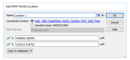
Geodesy
Geodesy is the science concerned with the measurement and mathematical description of the size and shape of the earth and its gravitational fields. Geodesy includes the large-scale, extended surveys for determining positions and elevations of points, in which the size and shape of the earth must be taken into account to achieve accuracy.
Vector vs Raster
The terms vector and raster are encountered often in cartography though they are not often defined. In a nutshell,
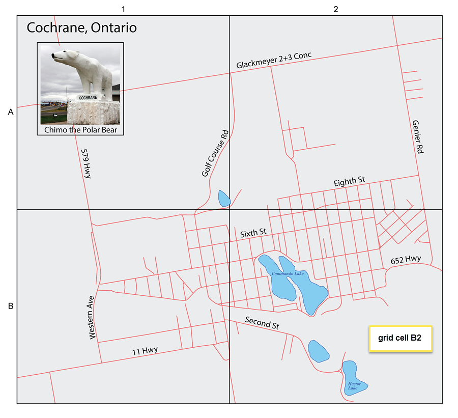
Raster data is made up of pixels (sometimes referred to as grid cells). Each pixel can have a range of values used to represent data points. For example, in a satellite image, every pixel has a red, green and blue value.
Vector data is not made up of a grid of pixels. Instead, vector graphics are comprised of vertices and paths where the vertices are x,y coordinates. In GIS systems, they are a latitude and longitude with a spatial reference frame.
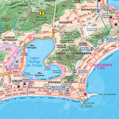
Mosaic
A Mosaic is a single raster dataset composed of two or more merged raster datasets—for example, one image can be created by assembling multiple aerial photographs whose edges usually have been torn or cut selectively and matched to the imagery on adjoining images to form a continuous representation of a portion of the Earth’s surface.
Orthorectification
The process of correcting the geometry of an image so that it appears as though each pixel were acquired from directly overhead. Orthorectification is used to correct terrain distortion in aerial or satellite imagery.
Sources
http://wiki.gis.com/wiki/index.php/GIS_Glossary/
https://legacy.lib.utexas.edu/maps/glossary.html
https://gisgeography.com/spatial-data-types-vector-raster/