Articles

New in MAPublisher 8.4: Import Map Data from Web Services

March 23, 2011

MAPublisher 8.4 has an exciting new feature: importing data from web services. It is another enhancement to provide you with more options to access data.

You can import vector data using the Web Feature Service (WFS). It accesses web servers that deliver vector content in GML format. Similarly, you can import raster data with the Web Map Service (WMS). It accesses web servers that deliver raster content in a variety of formats.

Access the WFS and WMS directly from the Simple or Advanced Import dialog boxes. After selecting either Web Feature Service or Web Map Service from the Format drop-down list, browse for a web service and select one. Of course, you can easily add, remove and manage your favourite WFS/WMS in this dialog box.

After selecting and connecting to a WFS/WMS, simply select features (layers) or rasters you want to import into Adobe Illustrator. At the same time, you will have an option whether or not to save the original datasets in GML format.

Click the Info button available next to the Server Info at the top of the dialog box. You can see more detail information about the web server.

After importing features from the WFS/WMS, each of the features will be in a MAP layer and all the georeferencing of those selected features will be stored in the MAP View.

New Text Utilities in MAPublisher 8.4

February 1, 2011

Among other great new features, MAPublisher 8.4 includes new text utilities designed to ease cartographic workflow by adding flexibility to text handling. These tools are accessed through two icons grouped with the MAPublisher document operations tools on the MAPublisher tool bar.

Text Utilities

Add functions like convert text on a path to point text, separate multiline text, extend overflowing text, flip upside down text, crop text path to text length, set text alignment, rectify point text to angle, and draw shape around text. These text utilities can be applied to selections, to layers, or to all document text at once. The following table provides examples for the result of each tool.

Right-to-Left Text Tool

Many right-to-left languages, such as Arabic and Hebrew, require additional language-specific processing to get the correct glyph output given the incoming character stream. Let’s look at an example.

Looking at the MAP Attribute panel, we see that the Arabic script is displayed properly

Yet, when using the Label Features tool, we see that the Arabic text is placed as a series of symbols that indicate that the text placement could not be accomplished accurately. This is one of two scenarios we will see, the other being that the Arabic characters will be placed left-to-right.

This happens because Label Features uses the currently selected font, in this case Myriad Pro. Since the Arabic characters were not found in the current Myriad Pro, the displayed symbol is substituted.

Once we apply the Right-to-Left text tool to these symbols, the Arabic characters will be reordered and altered to display the character appropriate to placement within the word and appropriate to surrounding characters. To apply the Right-to-Left text tool select Arabic from the preset drop-down menu. This populates the remaining settings with the correct parametrs.

Clicking OK, the script now matches what is found in the MAP Attribute Table.

If you are using MAP LabelPro, you will also need to use the Right-to-Left text tool after labeling. However, there is a slight difference between Feature Labels and MAP LabelPro behaviour. Instead of displaying the box with “x” symbol, it will place the Arabic characters in reverse order from their proper placement in the MAP Attributes table.

The text on the left is placed by MAP LabelPro, with the text on the right having been corrected with the Right-to-Left text tool.

We’re excited that these text utilities are being incorporated into MAPublisher. Many users have been requesting more text options. We hope you’ll like them as much as we do. We’re putting the finishing touches on MAPublisher 8.4 and will be releasing it in a few weeks.

Aligning data with different coordinate systems in MAPublisher

January 28, 2011

When first creating a map, very often you will find yourself having to align GIS data, especially if it is found or supplied by various sources. You might find that the coordinate systems assigned to each of the datasets might be different. This can prove challenging for many cartographers and GIS users. However, with MAPublisher, you can transform and align your datasets to one coordinate system very easily using the MAP Views panel.

For example, we have five layers with three different coordinate systems. After importing them into MAPublisher, the result is three different MAP Views. The MAP Area layer (Province) is in a Lambert conformal conic projection. The MAP Line Layer (river) and MAP Area layer (lake) are in a Robinson projection. Lastly, the MAP Point layer (cities) and MAP Line layer (roads) are in a geodetic coordinate system WGS84.

Let’s decide that the map we are creating here will have a Lambert conformal conic projection (the MAP View with the province area layer). Now, simply select the two layers in the Robinson MAP View, then drag them to the “Lambert Conf. Conic – 1: 30,000,000” MAP View.

The rivers and lakes layers are now transformed and aligned to the province boundary layer.

We will do the same for the cities and roads layers in the “WGS84” MAP View. Select the two map layers (cities and roads layers) then drag them to the “Lambert Conf. Conic – 1: 30,000,000” MAP View.

The cities and roads layers are projected on-the-fly. Now every layer is transformed to a Lambert conformal conic projection and aligned appropriately.

University of Montana Student Map Submissions

January 24, 2011

MAPublisher is popular with educators and students because, in no time at all, new users can begin to create great looking maps. Working seamlessly with the Adobe Illustrator environment, users can spend more time on map details and less time fighting with complicated importers and data format conversions.

Avenza Systems Inc. recently received student work submitted by the Univeristy of Montana’s Digital Design course. These maps show some excellent terrain shading, good colour choices, and a knack for making complex cartographic detail legible.

We wish to thank the students for generously allowing us to distribute their work, and we wish them luck in their upcoming mapping endeavours.

Click the maps to load high-resolution versions.

Buffalo Bill State Park Wyoming

by: Nathan Taylor

Crown of the Continent

by: Nathan Balding

Lolo Pass Recreational Trails

by: Hal Bobbitt

Georeferencing an Image in Adobe Photoshop with Geographic Imager

January 20, 2011

As of Geographic Imager 5.0, there’s an updated workflow for georeferencing images. Learn more about Georeferencing and work through the tutorial.

Nowadays, it’s common to find great orthophotos and satellite imagery on the Web. However, after downloading these (sometimes) large files, you might find that some don’t have any georeferencing. Most likely these files are in an image format supported by Adobe Photoshop(e.g. JPG or TIF) and you can georeference it using the Geographic Imager Georeference tool.

These are the requirements to georeference an image:

Knowing the coordinate system of the image (e.g. Mercator projection, State Plane system Alabama East, UTM system NAD 83 Zone 17 N..etc)
Finding three or more points from the image to assign coordinate values to each of them. These points are known as ground control points.

The first thing you need to know is the coordinate system or projection of the image you are georereferncing. If you are unsure about which coordinate system the image uses, contact the data provider or search the metadata of the image on the Internet. If you cannot get the information of the coordinate system assigned to the image, you might want to try georeferencing with different coordinate systems to make the map as precise as possible.

The second requirement is working with the ground control points. One ground control point consists of several values: 1) Pixel X coordinate, 2) Pixel Y coordinate, 3) Ground X coordinate (e.g. longitude), and 4) Ground Y coordinate (e.g. latitude). Furthermore, to make georeferencing easier, ground control points must be clearly identifiable in the image. Cultural features such as road intersection, a sharp corner of a lot or boundary are good examples of locations used as ground control points.

Now that you know what you’ll need, we’ll demonstrate a georeference workflow using the Geographic Imager Georeference tool and Google Earth.

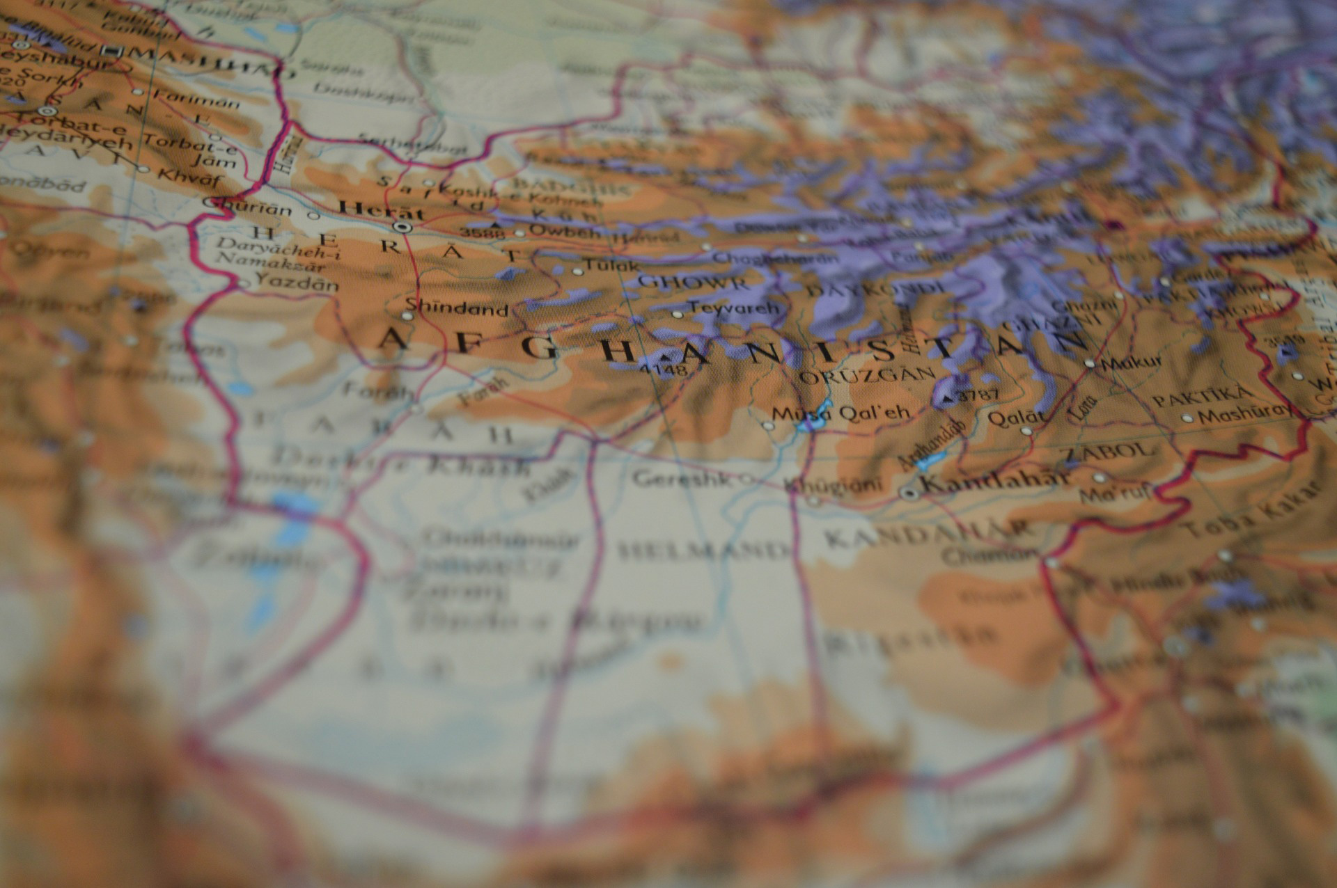
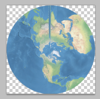
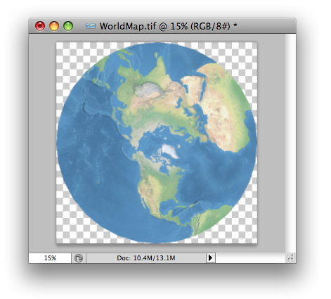
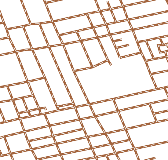
Step 1: Obtain a non-georeferenced image

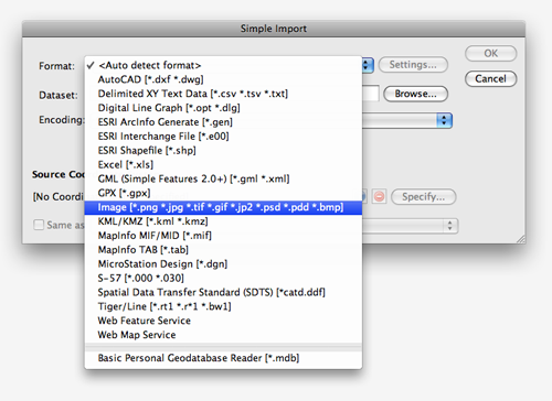
This image is in JPEG format and there is no georeference information associated with it. In order to transform it to another coordinate system or projection, mosaic with other images, or align the image to vector work using MAPublisher for Adobe Illustrator, the image must first be georeferenced.

Step 2: Obtain the required information

As indicated above, two key pieces of information are required to georeference an image: a) the coordinate system of the image and b) defining ground control points

a) The coordinate system of the image

The image, collected from Google Earth, is projected in a coordinate system called WGS84 / Pseudo Mercator (this projection is common to Web based mapping systems and is also known as Web Mercator or Google projection).

b) Defining ground control points

We’ll need to define at least three ground control points for georeferencing. Below are the steps for finding out one of the ground control points.

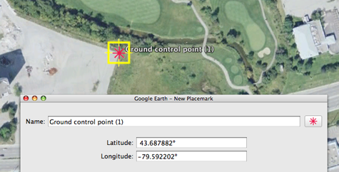
On the non-georeferenced image, decide which spot to use as a point of reference. It should be available on Google Earth where you’ll find the X,Y coordinate values. For the first point, we’ll use the corner boundary between the pavement and a golf course.

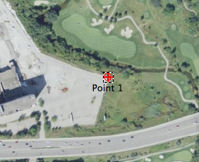
Using Google Earth, find the exact same spot as the one decided in the non-georeferenced image. Place a point symbol to help identify the coordinate values. Record the collected latitude and longitude values. The latitude and longitude values are at the centre of the point symbol in the Google Earth window.

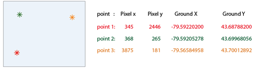
Find the coordinates of two additional ground control points. The latitude and longitude values are in decimal degree format and the coordinate system of those values are in the geodetic system “WGS84”.

Step 3: Georeference in Geographic Imager

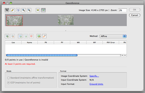
In Geographic Imager, click the Georeference tool button in the Geograhpic Imager main panel (or choose File > Automate > Geographic Imager : Georerence). The Georeference dialog box will open.

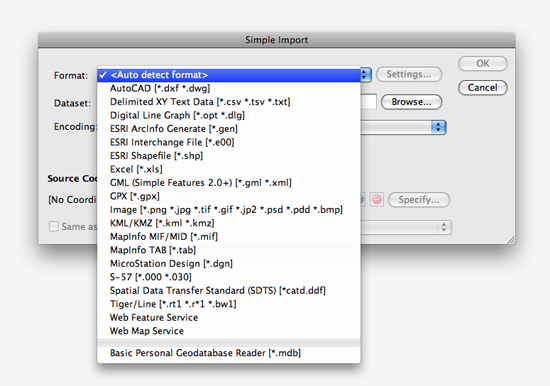
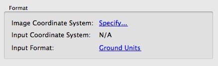
First, we’ll need to set the proper image coordinate system and input coordinate system (the information from Step 2a). In the Format section, click the blue “Specify” link to open the Input Format dialog box.

Here we’ll specify two parameters: Image Coordinate System and alternate input coordinate system. The image of the coordinate system is WGS84 / Pseudo-Mercator as found at Step 2a. Click the “Specify” button to find the coordinate system from the coordinate systems list.

The option “Use alternate input coordinate system” will not have to be selected if the X,Y coordinate values are collected in the Eastings/Northings in the WGS84 / Pseudo-Mercator coordinate system. When those latitude and longitude values are collected, those values are collected in the decimal degree format and the values are in degree in WGS84. We will use those latitude and longitude values for the georeferencing. Specify the destination coordinate system as WGS84.

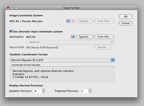
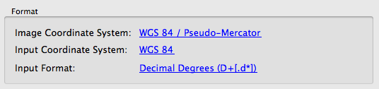
When the settings are made, click OK to close the Input Format dialog box. All the selected coordinate system for each setting will be indicated in the Format section of the Georeference dialog box.

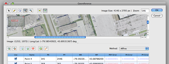
The next step is to enter the three ground control points collected from Google Earth. Click the pencil tool at the top of the Georeference dialog box and click a point for one of the ground control points collected at the previous steps .

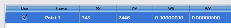
As soon as one point is clicked on the preview image, it will add one row in the Georeference table. This row contains the point name, PX (Pixel x coordinate), PY (Pixel y coordinate), WX (World X coordinate), and WY (World Y coordinate).

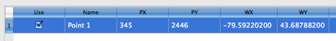
For WX and WY, enter the longitude and latitude, respectively, for the first ground control point.

Repeat the same steps for the second and third ground control points.

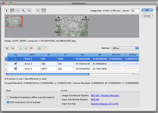
As soon as you enter three points, Geographic Imager will display the residual error values on the table for the accuracy assessment.

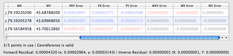
A residual error is the computed difference between an observed source coordinate and a calculated source coordinate. It is the measure of the fit between the true locations and the transformed locations of the output control points. A high residual error indicates possible error in either the observed source coordinates or the reference coordinates of the reference point in question.

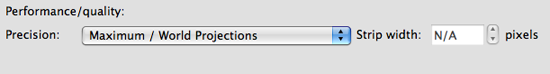
When the error is particularly large, you may want to remove and add control points to adjust the error. As a general rule, apply several different transformation methods, select/deselect questionable points and select the method and reference points that yield the minimum residual error, assuming that the defined reference points are correct. Residual values are calculated via the associated error values between computed values and entered values through either the affine or various polynomial methods.

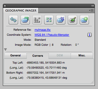
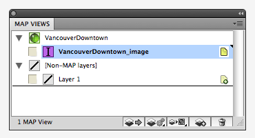
Once completed, the Geographic Imager main panel will indicate the georeference information of the image. Don’t forget to save the file once it is complete. Now your image is ready for any Geographic Imager function. You can also bring this image into MAPublisher for Adobe illustrator and align it to other GIS data.

New in MAPublisher 8.4: Image MAP Layer feature type for georeferenced images

January 17, 2011

MAPublisher 8.4 introduces two new related features: to import supported image formats directly from the MAPublisher Simple and Advanced Import dialog boxes and the Image MAP Layer feature type. To import a georeferenced image into the current MAPublisher 8.3 (and earlier) requires you 1) to create a new MAP Layer for an image to be placed, 2) use File > Place to place an image into the Adobe Illustrator document, and 3) to use MAPublisher Register Image to align with the vector work. With MAPublisher 8.4, these steps are streamlined and it will be much simpler to deal with georeferenced image files.

Below is the Simple Import dialog box. The new Format option, Image, is added to the drop-down list. Supported images include: PNG, JPG, TIF, GIF, JP2, PSD, PDD, and BMP.

The VancouverDowntown.tif file was selected from the MAPublisher Quick Start dataset. The source coordinate system of the image, “NAD 83 / UTM Zone 10N”, is automatically detected because it is a GeoTIFF and contains the georeference information of the image.

When the georeferenced image is imported by MAPublisher, it is stored in a new layer called “VancouverDowntown_image”. MAPublisher 8.4 introduces a new MAP Layer feature type called “Image”, a purple icon with the letter ” I “. From now on, all images should be placed on Image MAP Layers.

Remember that images placed in Adobe Illustrator using MAPublisher cannot be transformed or reprojected into another coordinate system. To transform an image from one coordinate system to another, it must be done using another software such as Geographic Imager.

MAPublisher 8.4 will be released very soon. Thanks for sending us feature requests like this one. If you have any feature requests for MAPublisher, Geographic Imager or PDF Maps, please feel free to drop us a line at support@avenza.com. We’re always happy to hear from you!

How to Download USGS Maps for your iPhone, iPad or iPod Touch

January 11, 2011

If you haven’t read about it yet, USGS topographic maps for the United States are now available for download on the Avenza PDF Maps Library.

USGS topographic maps are great for viewing, reference and recreational uses such as hiking, fishing or exploring. You can download the maps beforehand (in cellular range or over Wi-Fi) and use the GPS capability (of the iPhone and iPad Wi-Fi+3G) to locate yourself on the map. These 1:24,000 scale maps include the lower 48 states, Alaska, Hawaii and the District of Columbia. All of the maps are in geospatial PDF format. Best of all, majority of the maps are lightweight meaning they download and process quickly on your device.

The process of getting USGS maps on your iOS device is simple

First, download and install the app if you don’t have it yet. Open the PDF Maps app. In the map list screen, tap the + button (Add Map) in the top-right corner.

Then tap the From Avenza PDF Maps Library button.

The app connects to our PDF Maps Library server and lists several categories. Tap the USGS Topographic Maps category.

The maps are categorized by state and area. We’ll retrieve a topographic map of a part of the city of Tucson, AZ. In the list of the U.S. states, tap Arizona.

In the preview map of Arizona, area grids are represented by the dashed gray lines. These area grids contain all of the available topographic maps categorized further by area name. Tap the area grid that contains Tucson.

Scroll down the list and tap Tucson East. This will take you to a preview of the map before the last step of downloading it.

A preview of the map is shown. Finally, tap the Download 3.3MB button to download the Tucson East map. The PDF file size is listed as 3.3 MB.

The device automatically returns to the PDF Maps app where the Tucson East map will be downloading. After the download is complete, the app will automatically process and render all the tiles you’ll need to explore the map. This will only take a few minutes.

When the processing is completed, it will show it’s total size (18.1 MB) that includes tiles for all of the different zoom levels. Tap the Tucson East map to load it.

These USGS maps and other maps on the Avenza PDF Maps Library are fully georeferenced and compatible with PDF Maps. Still have questions about PDF Maps? Read our support page or send us your questions. Stay tuned for more content.

New Join Areas feature in MAPublisher 8.4

December 28, 2010

The upcoming release of MAPublisher 8.4 introduces many new features. One of the new features is called Join Areas. We have received a lot of requests from our customers to create area objects by merging common attribute values. This geoprocessing function is generally known as “dissolve”.

The picture below shows polygon objects from a USA Counties layer. The goal is to create a layer with state boundaries and summing the population count by joining the objects of the counties layer.

In the MAP Attributes panel of the USA Counties layer, every object of the counties layer contains attribute information including county name, state name, FIPS codes, area in km², population and so on. We’ll be using the StateName attribute value to combine all the county polygons into one polygon per state.

This is the new Join Area dialog box. On the left side, we’ll specify 1) target layer, 2) destination (output) layer, 3) join type and 4) join method. We are trying to create state boundaries from the counties target layer so we’ll select a join type based on the StateName attribute and output it to a new layer called USA States. The join will create compound paths and since our goal is to create state polygons, we’ll dissolve borders between adjacent sub-areas.

On the right side of the dialog box are attribute value operations available for each column. These operations determine what kind of the values will result for every attribute and the operations available are different for each data type (String, Real, Integer). The screenshot below shows the attribute value operation set to Sum for Population attribute (Integer data type). When the Join Area is complete, each state polygon will have the sum of the population of all the counties that belong to it.

After running the Join Areas function, county polygons are dissolved into state boundaries.

The population values show the total sum from all the counties for every state.

This is just one example of how Join Areas can be used. It was initially a feature request and with some discussion and planning, it became real. If you have any feature requests for MAPublisher, Geographic Imager or PDF Maps, please feel free to drop us a line at support@avenza.com. We’re happy to hear from all of you!

New Transformation Method for World Maps in Geographic Imager 3.2

November 29, 2010

When transforming a world image, there may be artifacts created by the Geographic Imager transformation engine. Below are the results of a WGS84 world image transformed into a Stereographic projection.

When we zoom into the problematic area, you can see up close how some artifacts affect the image after the transformation was performed.

To solve this issue, we are introducing a new projection method called Maximum: World Projection in Geographic Imager 3.2.

We are going to use the same world image used with the previous example and transform it into the stereographic projection. Take a close look at the Advanced Options.

Under the Performance/quality section, select Maximum / World Projections from the Precision drop-down list and click OK.

Below is the result of the transformation with the new method available in Geographic Imager 3.2.

Let’s take a close look at the same area where the problem happened with the previous version of Geographic Imager. Now the transformed image does not contain any artifacts.

This option is available since Geographic Imager 3.2. The official version of Geographic Imager 3.2 is available now.

Making dashed lines intersect at every intersection in MAPublisher

December 7, 2010

One of the great advantages of using Adobe Illustrator for a mapping project is that you can make great line styles easily. For example, to make a double line stroke and one of them is dashed:

Double strokes are a line graphic style where two different line strokes overlap each other. For example, the image shows that there is a stroke with a brown color and its stroke size is 3 pts. On top of this brown line, there is a 1 pt white dash line:

You might have an experience where you duplicated one line layer and assigned a different style for lines in each of those layers. However, this has some disadvantages. The file size will increase because all the line segments as well as the attribute information attached to every line object is duplicated. Also, when you apply the double stroke line to road layer, the white dash line does not intersect nicely at every intersection of the map:

With Adobe Illustrator CS5, these problems are solved.

0) Create a graphic style like the one shown above.

1) Open the Pathfinder panel (Window > Pathfinder).

2) Select all the line objects in the line layer.
Click the outline tool .

This function in the Pathfinder tool breaks lines at every intersection.

All the selected objects which were selected at Step 2 will be broken into segments at every intersection and they will be grouped as one object in the layer.

3) Having the grouped objects selected, apply the graphic style with the double stoke.

4) The white dashed line is intersected at every intersection nicely.

Quick tip

When creating double stroke, make sure to select the option “Align dashes to corners & path ends, adjusting length to fit” available next to the dash line option.

Note

Since this operation involves a pathfinder functions, the attribute information will not be matintained after the “outline” function is applied to those selected line works. Our development team is looking for a possible solution to keep the attribute information for the future version of MAPublisher.

Avenza maps makes it easy to interact with offline
maps on your iOS, Android and Windows devices.