This guest blog post was written by Tom Patterson — one of the creators of the Equal Earth Projection, and Natural Earth Data, (you can read more about Tom here). Learn how he used Geographic Imager for Adobe Photoshop to create two maps from Landsat 8 imagery.
I am a big fan of Landsat 8 satellite images as a resource when making maps. Typically, I use these free images taken every 16 days for verifying and updating other geospatial datasets. I also transfer Landsat textures to shaded relief art in order to better evoke a sense of the physical environment.
The examples that follow demonstrate how I have used Landsat imagery to enhance two maps. The first example is Prince William Sound, Alaska, a map that I am presently working on. The second example is a Landsat mosaic of the Big Island of Hawaii. Both of my examples will give you a general idea on how to integrate Landsat images into your cartographic workflow—using Avenza’s GIS plugins for Adobe Photoshop and Illustrator—with a few technical tips thrown in for good measure. For in-depth information about using Landsat in Photoshop, refer to this tutorial.
Prince William Sound, Alaska
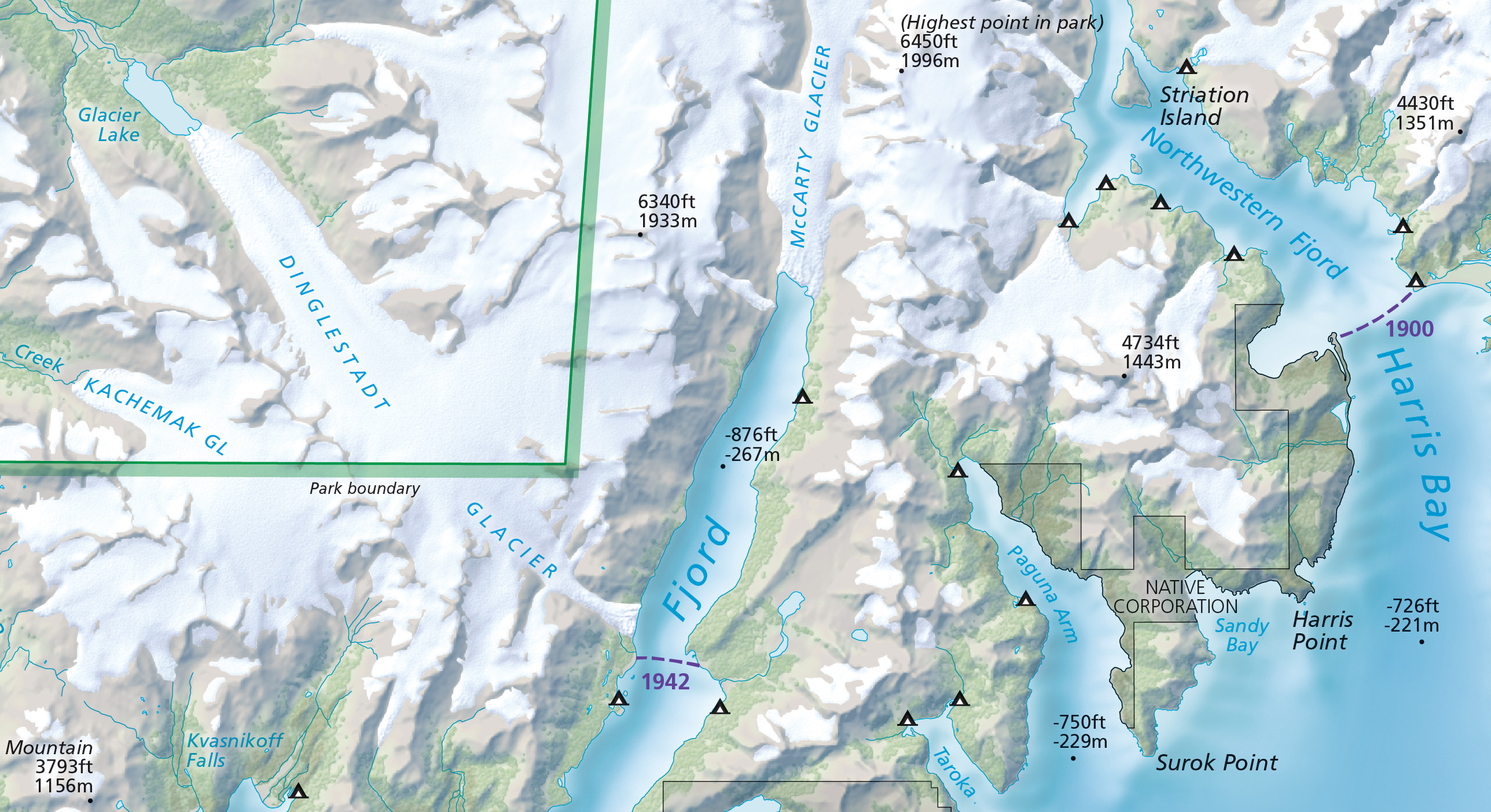
Prince William Sound, in south-central Alaska, is a spectacular place to map. Its sheltered waters are bounded by the lofty Chugach Mountains, indented by deep fjords with tidewater glaciers, and dotted by forest-cloaked islands. The problem I am facing is out-of-date geospatial data because of the rapidly melting of glaciers. For example, the positions of glaciers, lakes, rivers, and coastlines available in the National Hydro Dataset (NHD) have changed considerably since these data were collected between 2008 and 2012. In order to make an accurate map—if only for this year—I have had to re-digitize these vector elements using Landsat images as a reference.
For this task, I used “LandsatLook Images with Geographic Reference” downloaded from the Earth Explorer website. These quasi-natural color images, which come pre-made from bands 7, 5, and 3, clearly depict water bodies, vegetation, bare earth, and glaciers. They were perfect for mapping the changing landscape of Prince William Sound.
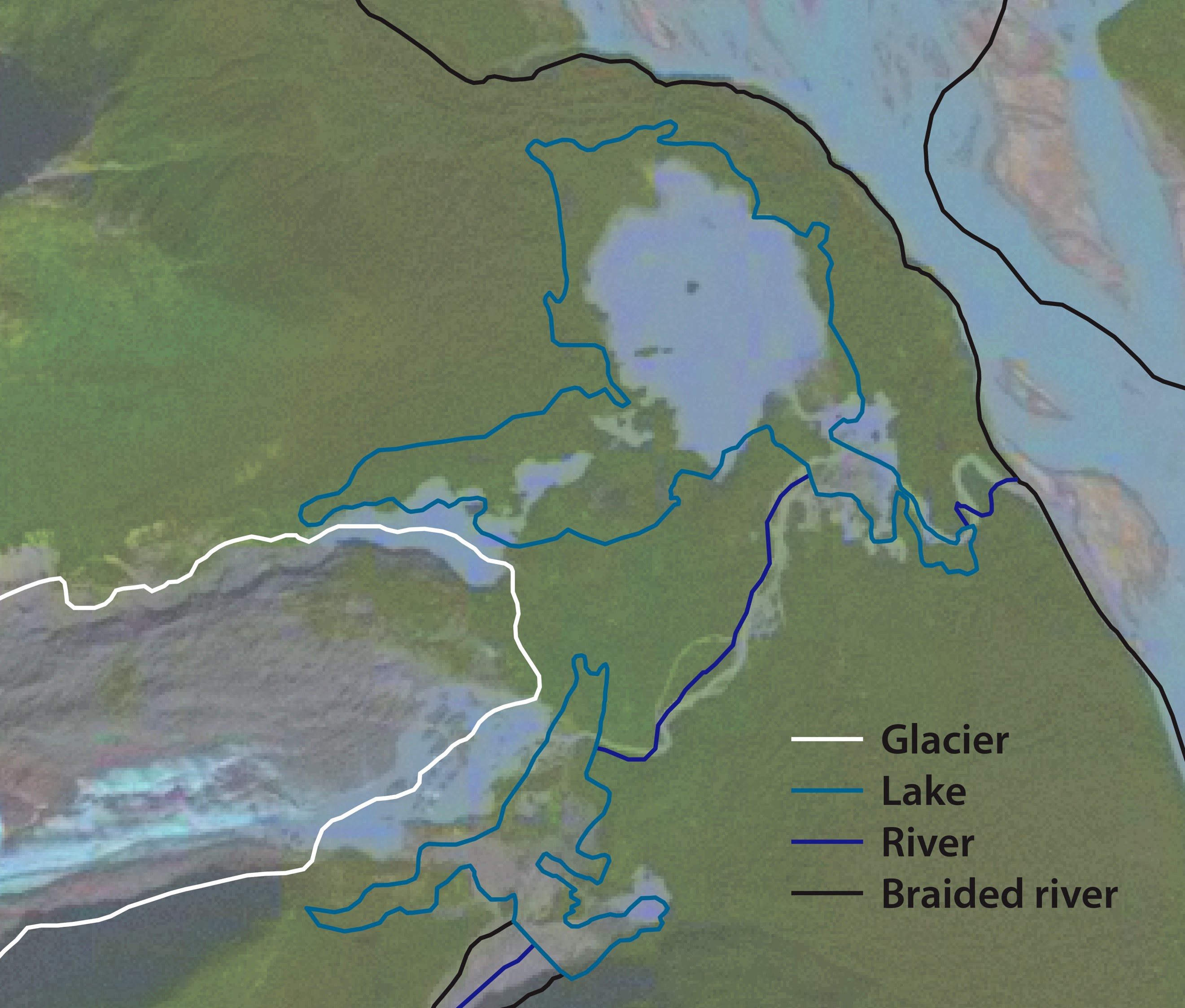 National Hydro Dataset lines overlaid on a LandsatLook image in Adobe Illustrator.
The lines do not match physical features on the more recent satellite image.
For reference, I used images taken on September 29, 2018, about the time when glacier melting ceases before the onset of winter. Images taken later in the fall are hampered by fresh snow cover and deep mountain shadows due to lower sun angles.
Because the LandsatLook images were in the same projection as my map, I could directly place and then register the images in the Adobe Illustrator file with MAPublisher. Had the projections been different, I first would have had to transform the LandsatLook images using the Geographic Imager plugin in Adobe Photoshop. Finally, I moved the LandsatLook images to a bottom layer and dimmed them for editing the lines with Illustrator’s Pencil tool. Using a Wacom tablet and stylus for editing lines greatly improved my drawing speed and accuracy.
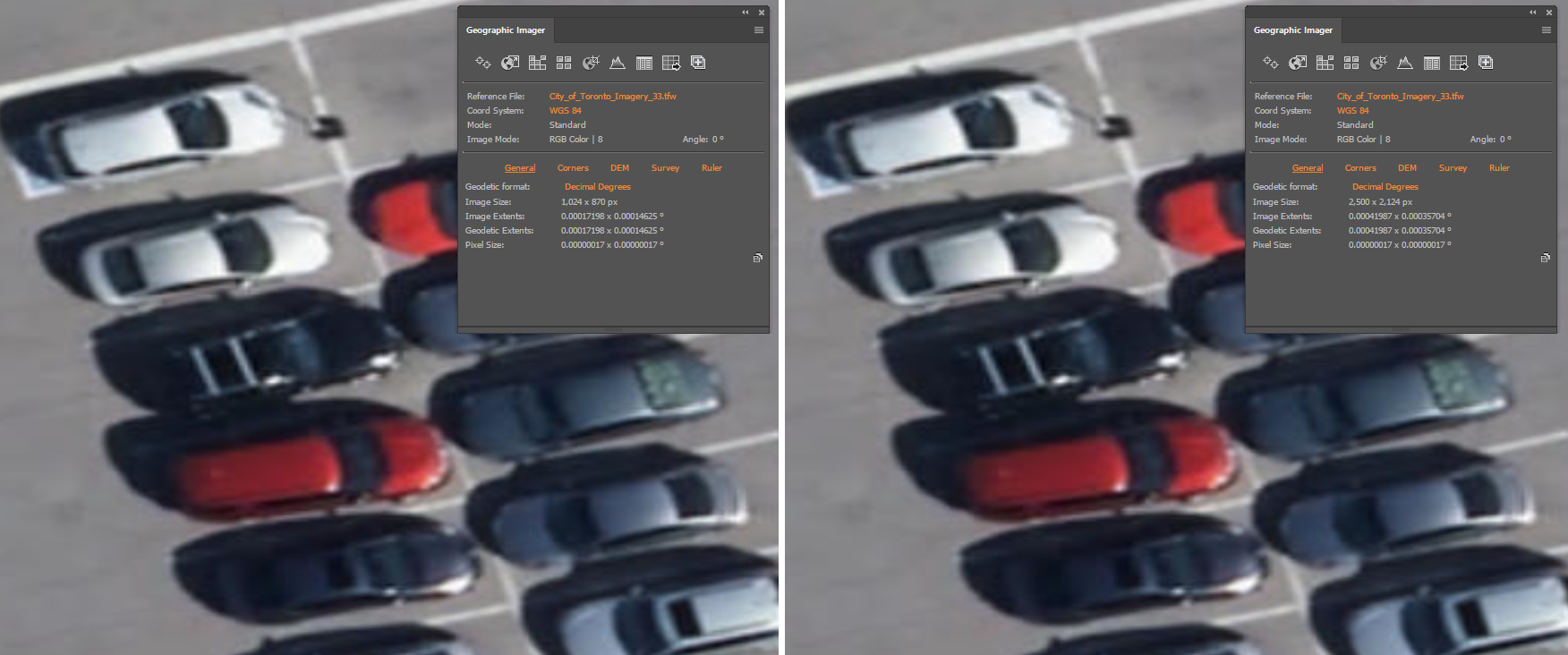
If a 30-meter LandsatLook image lacks enough detail, you can increase the apparent resolution to 15 meters by applying panchromatic sharpening. Doing this will involve downloading all data bands that comprise the Landsat scene (a Zipped archive about 1 GB in size). Within this archive is Band 8, a grayscale image showing the same area as the LandsatLook image, but with double the resolution.
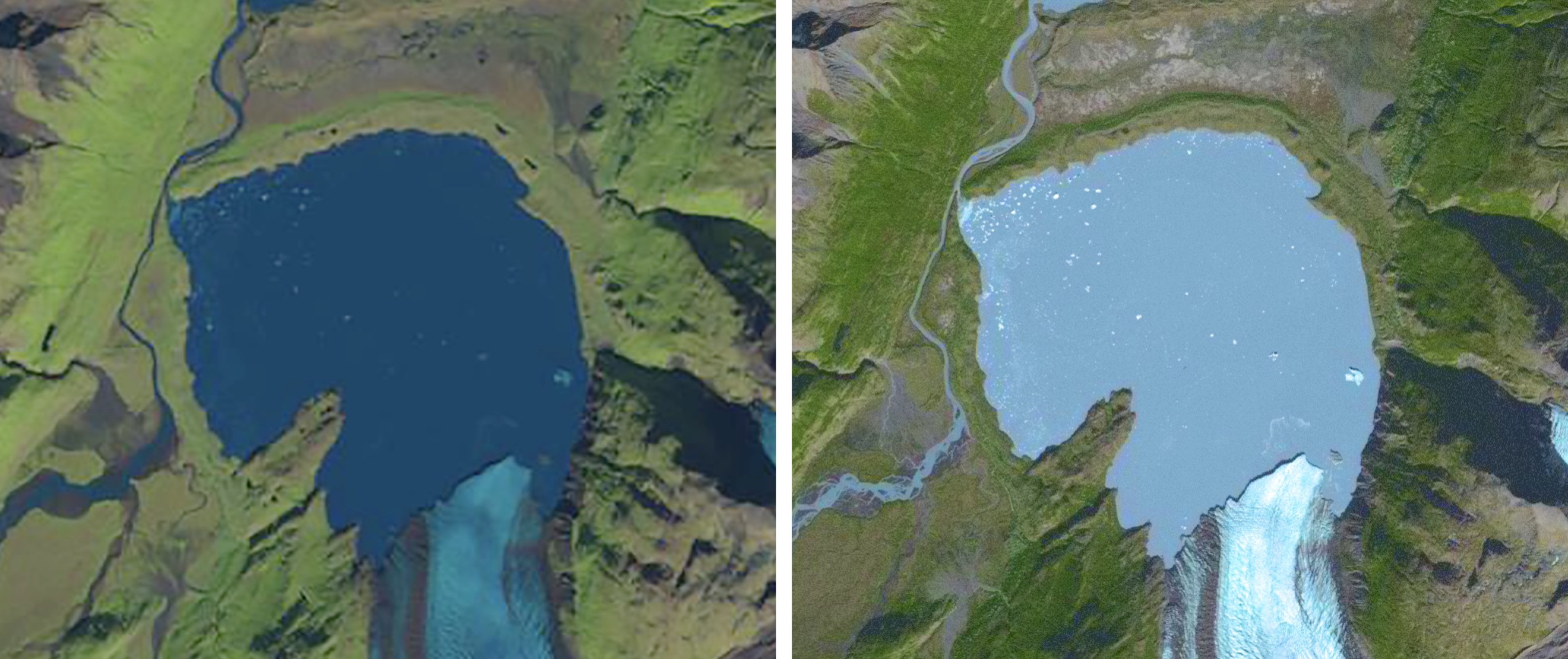 Coming into focus. A LandsatLook image before (left) and after (right) panchromatic sharpening.
Besides increasing detail, panchromatic sharpening also shifts colors.
Once Band 8 is downloaded, the first step is to enlarge the size of the LandsatLook image by 200 percent in Photoshop (Image/Image Size). Resample it using the Preserve Details (enlargement) option. Next, copy and paste Band 8 on top of the LandsatLook image. Then, in the Layers window, change the blending mode of the Band 8 layer from Normal to Luminosity. Finally, apply Curves adjustments to both layers until the tonal range of the combined image is to your liking. The pan-sharpened LandsatLook image will keep its georeferencing thanks to the Geographic Imager plugin.
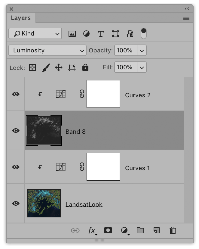 Use the Layers window in Photoshop to apply panchromatic sharpening.
Selecting Luminosity blending mode for the Band 8 layer is key.
The Big Island, Hawaii
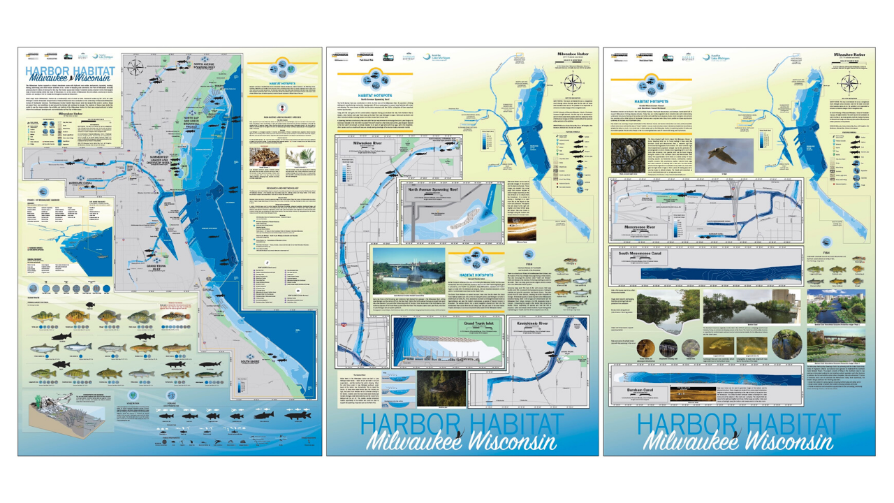
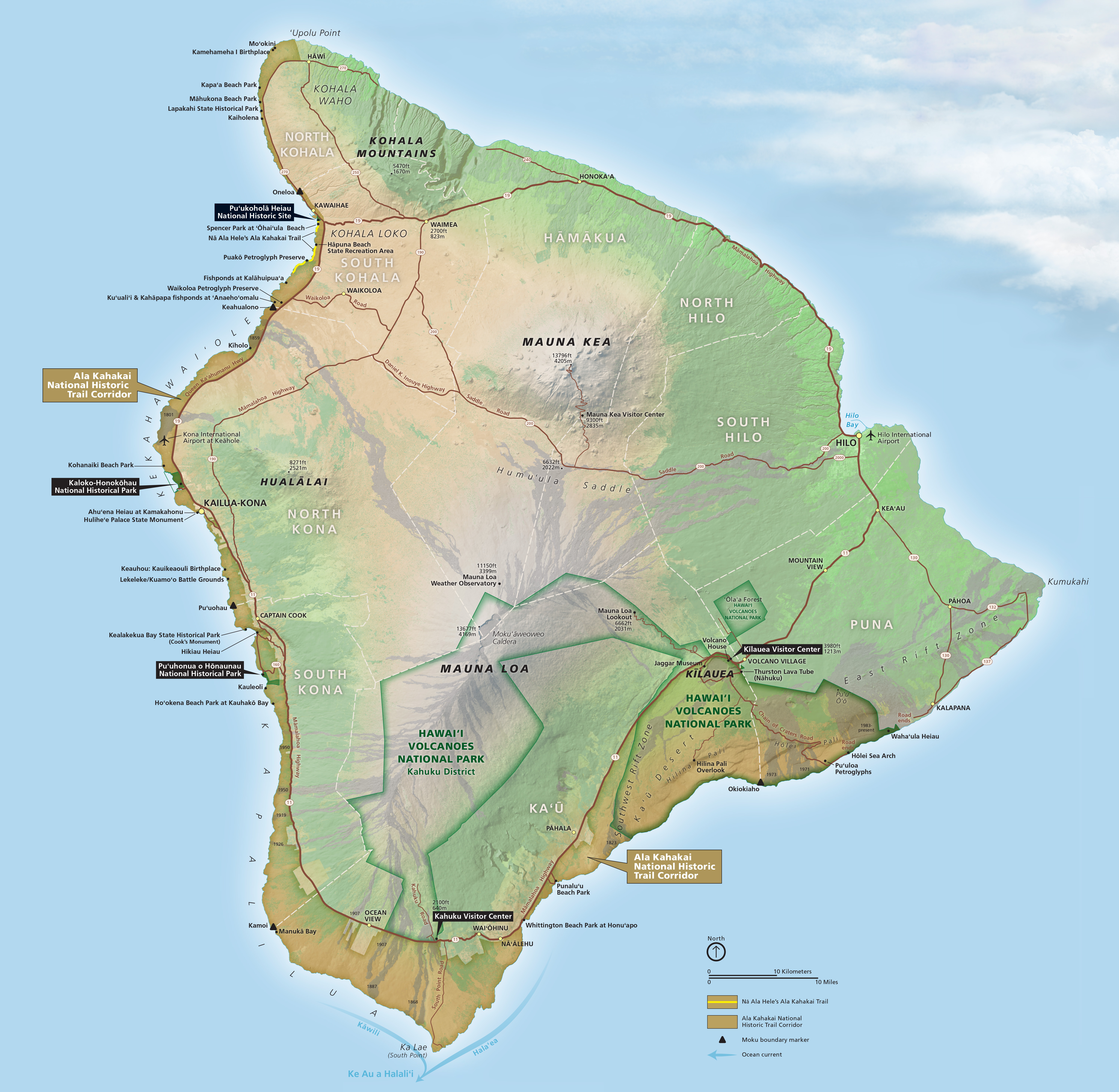
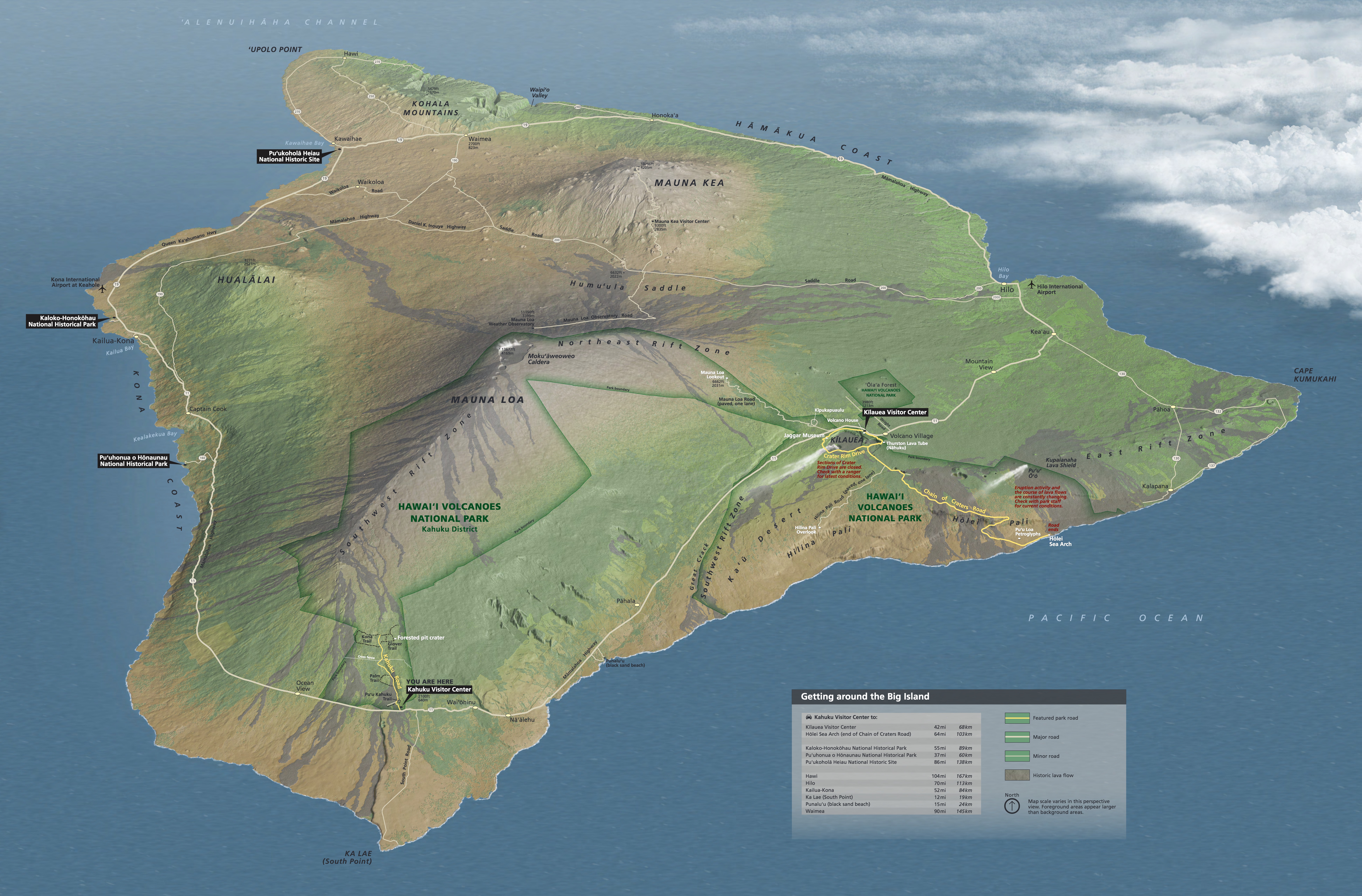
In 2017, I created a Landsat mosaic of the Big Island as a starting point for making two National Park Service maps: Ala Kahakai National Historic Trail and Hawaii Volcanoes National Park. I used the Landsat mosaic as a source for land cover textures—forest cover and historic lava flows (those that formed since 1800)—depicted on these maps. Compared to the Landsat mosaic, the map textures print very lightly in the interest of visual cleanliness.
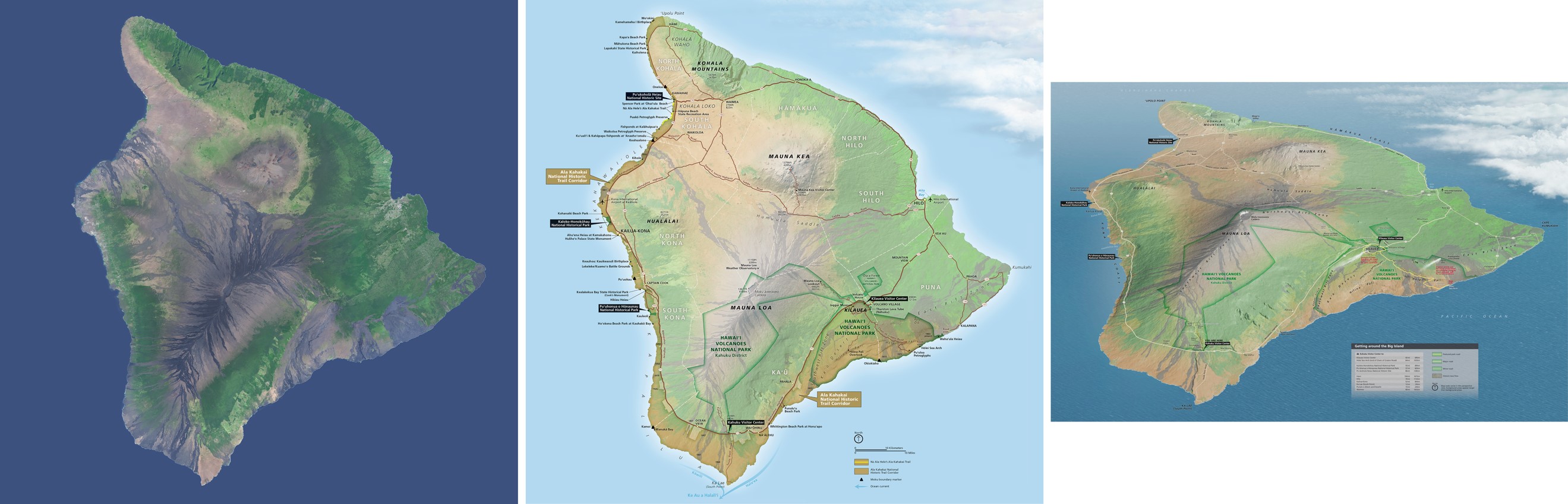 Big Island Landsat mosaic (left) and the maps of Ala Kahakai National Historic Trail (middle) and Hawaii Volcanoes National Park (right) derived from it. Click here to see a larger version of the Ala Kahakai map (5 MB) and here for the Hawaii Volcanoes map (6.4 MB).
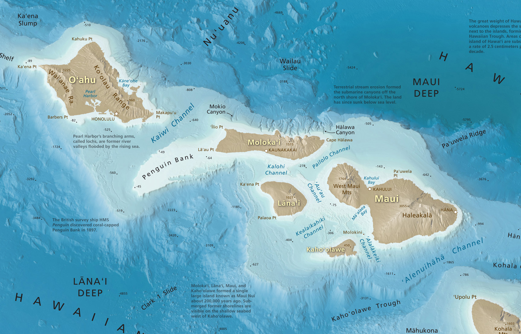
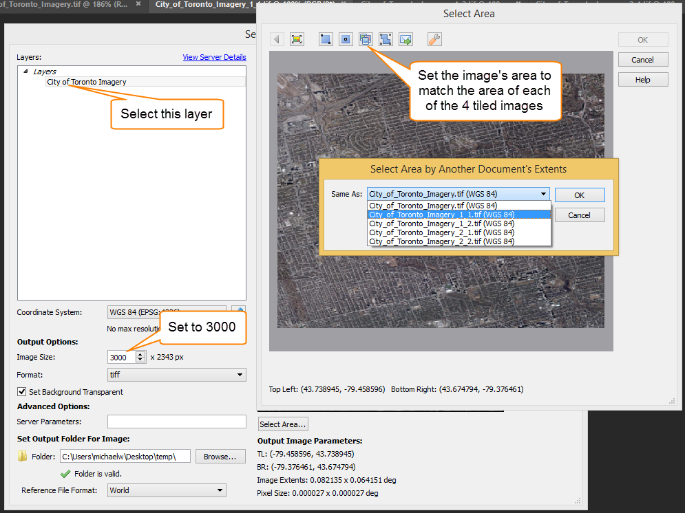
The first step in creating a Landsat mosaic was downloading the appropriate image data. In a perfect world, a mosaic of the Big Island would only require four 185-kilometer-wide Landsat images. However, because of persistent cloudiness on the windward side of the island, ten images were needed to complete a nearly cloud-free mosaic. Using images taken in previous years was a necessity. When selecting older images with fewer clouds, I looked for those taken at about the same time of year to keep the lighting consistent. I then used the Clone Stamp and Spot Healing Brush tools in Photoshop to carefully delete any unavoidable clouds and their shadows from the mosaic. Fortunately, the few clouds that remained were in remote areas far from the main focus of the final maps.
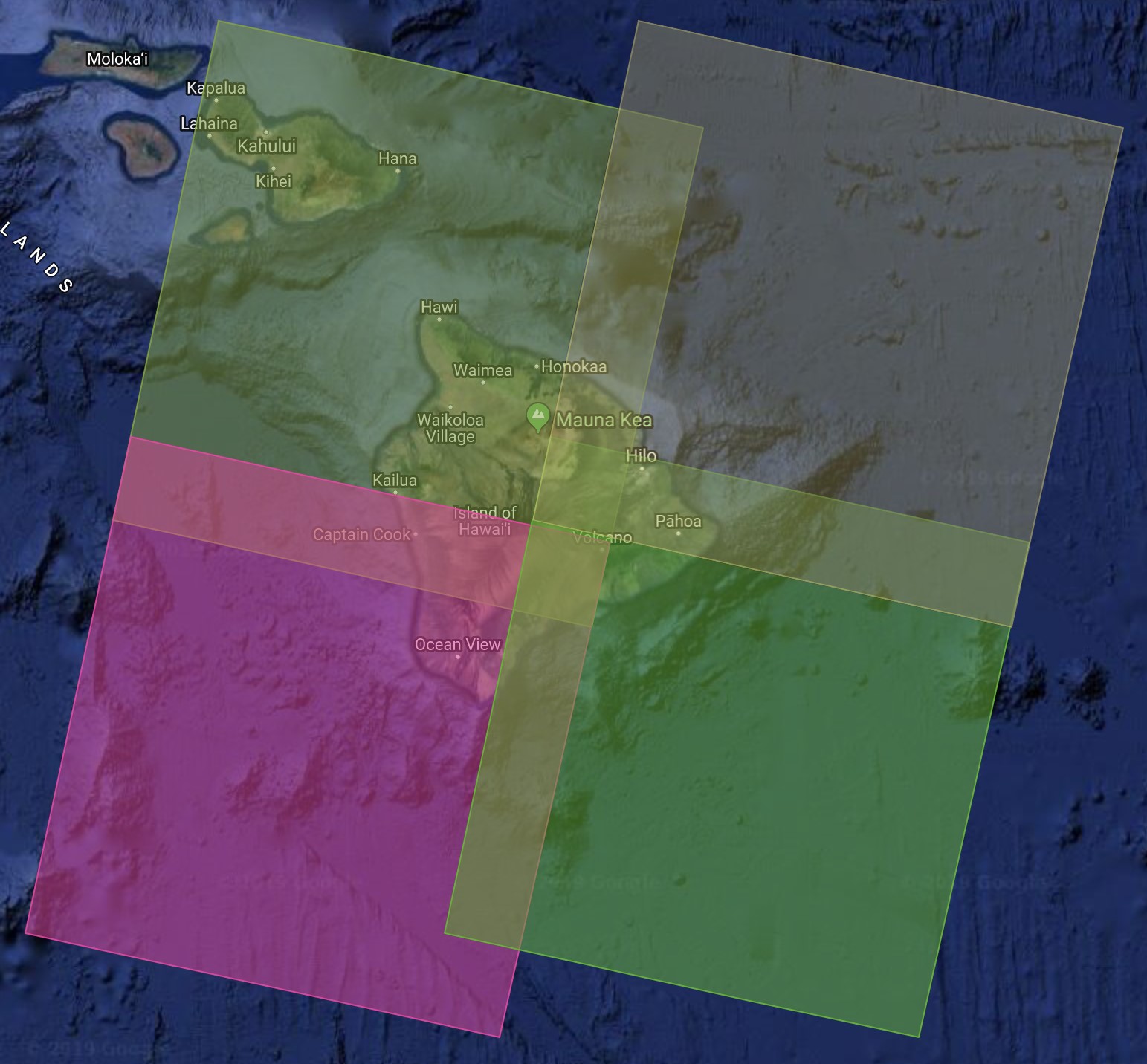 The Big Island is covered by four overlapping Landsat images.
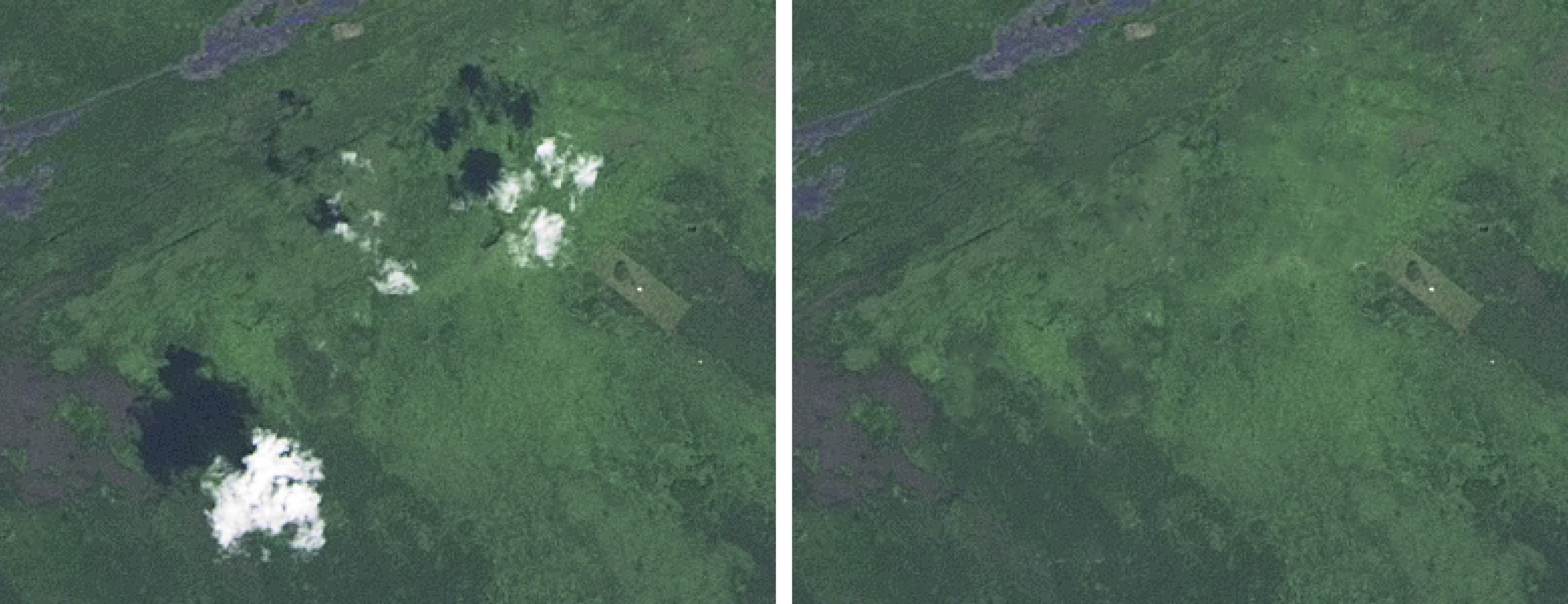 Clouds be gone. The Landsat mosaic before (left) and after (right) editing.
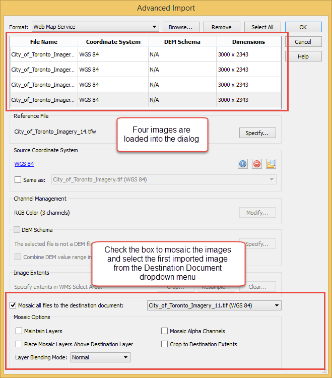
The Landsat mosaic was assembled in Photoshop using Geographic Imager (File/Automate/GI: Mosaic). In the Mosaic window, I selected the Maintain Layers option to ensure that each Landsat image was placed on a separate layer. I then added layer masks to each image layer to piece together the ten images with the goal of avoiding clouds. Although the masks themselves with feathered edges looked like a messy jig-saw puzzle, they combined to produce a seamless Landsat satellite image mosaic.
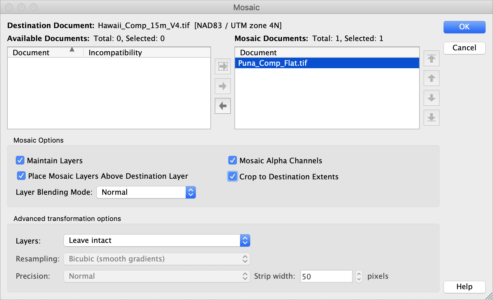 Geographic Imager’s Mosaic window.
I created the Big Island mosaic in natural color by compositing Bands 4, 3, and 2 as red, green, and blue channels, respectively, in Photoshop. I also brightened the forested areas with LandsatLook mosaic placed on the topmost Photoshop layer and with the layer opacity reduced (in normal blending mode). The natural color procedure is explained in detail here.
With a Landsat mosaic of the Big Island completed, my next task was extracting the forest and lava textures and applying them to the Ala Kahakai and Hawaii Volcanoes maps. But that was an involved procedure that will have to wait for another blog.
One more thing …
Since making the Big Island mosaic in 2017, the Puna district experienced volcanic activity in 2018 that covered a large area in lava and reconfigured the shoreline. Although Puna is the cloudiest area on the Big Island, I was lucky to find a recent cloud-free Landsat image that I then used to update the mosaic. You can download a GeoTIFF of the updated mosaic here (120 MB). It is in the public domain.
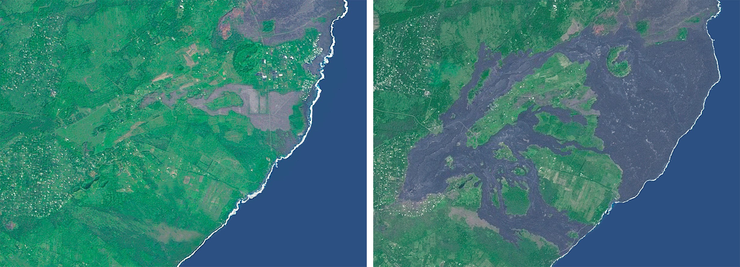 Puna District, Hawaii, before (left) and after (right) the volcanic eruptions of 2018.


