Original article from Directions Magazine on October 4, 2017.
Modern cartography—the art, science, and technology of making maps—consists of manipulating and displaying geographic elements in a graphic environment. Traditionally, GIS software has offered users limited ability to manipulate the graphic attributes (hue, brightness, saturation, transparency, line thickness, text, etc.) of geographic elements, while graphic design software has treated geographic features as it would any other graphic elements, without regard for how they are connected in predictable ways to other geographic elements and to Earth itself. Additionally, in the real world, natural or artificial boundaries and features are constantly changing and cartographers need to update maps at different scales and in different styles to reflect these changes. Therefore, cartographers need an efficient and reliable way to bridge the divide between GIS and graphic design software.
First launched 30 years ago, Adobe Illustrator has long been the professional standard for graphic design, especially for creating vector graphics. For more than 20 years, Avenza’s MAPublisher has provided extensive GIS functionality inside Adobe Illustrator. I discussed the synergy between these two programs with two experts:
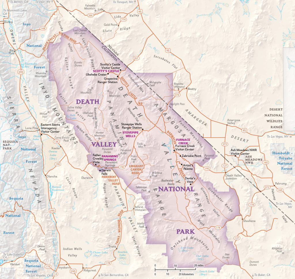
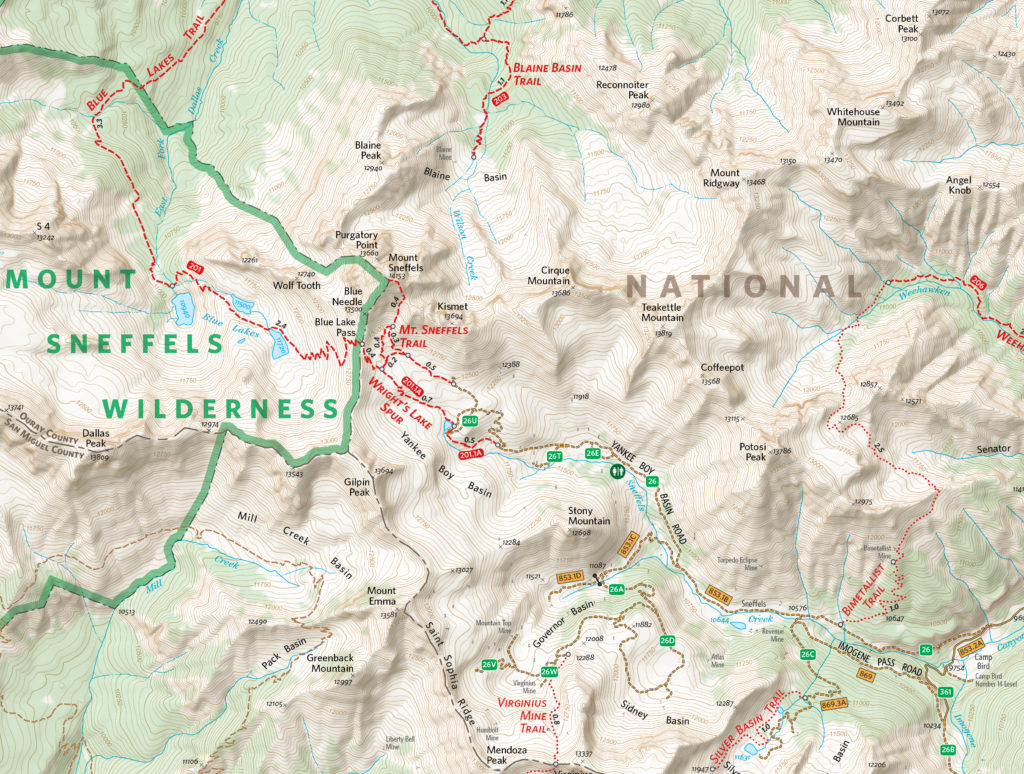
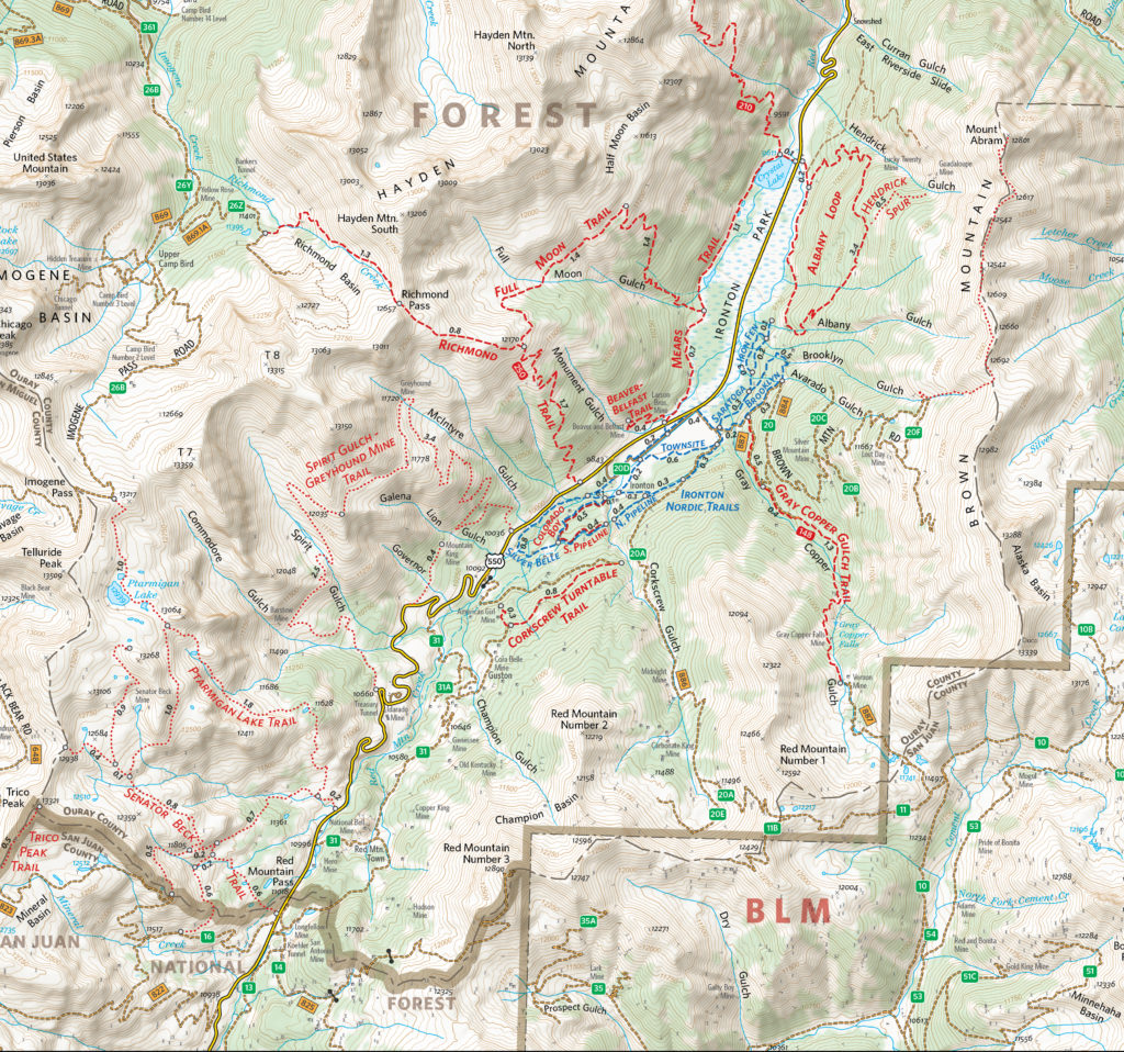
- David Lambert, Director of Cartographic Production for National Geographic’s commercial retail mapping products, which includes its well known Trails Illustrated outdoor recreation map series, and
- Tom Patterson, Senior Cartographer at the National Park Service’s Harpers Ferry Center, in Harpers Ferry, West Virginia, which designs most of the interpretive media that is found in national parks—including maps, brochures, outdoor signs, visitor center exhibits, films, and digital kiosks.
“Map Illiterate” vs. “Map Aware”
In the past, many map makers have also used Macromedia FreeHand (acquired by Adobe in 2005 and since discontinued), CorelDRAW, Canvas, or even more recent entrants with a map-specific slant such as Ortelius, proving that a graphics environment has long been regarded as a good and viable one for their trade. As well, for many years, Esri has offered an Illustrator export option from its GIS products, proving that Illustrator, in particular, has long been the preferred work environment for making maps. However, Lambert points out that those files exported from Esri’s GIS products are devoid of geographic properties once imported into Illustrator. He has been with National Geographic for 21 years. His team used to work with Illustrator, which was already the graphic design standard, but used Esri software to design maps, which they then exported as Illustrator files from Esri and imported to Illustrator. “Once we brought that into the Illustrator format, it lost all geospatial awareness,” Lambert recalls. In essence, the file became “map illiterate.” In 2011, he switched to using MAPublisher after learning how easy it made it to incorporate GIS data into Illustrator workflows.
To explain the advantages of using MAPublisher to keep graphic elements “map aware”, Lambert cites three examples:
- The Great Salt Lake has shrunk in size over the years. “Prior to 2010, somebody would export a lake boundary and then bring it into Adobe Illustrator, where it might be re-scaled and transformed with an Illustrator function to fit the area of another map,” Lambert recalls. Now, with MAPublisher, National Geographic can use the same lake boundary in its maps of Utah, of the United States, and of the world, in each case simply reprojecting it on the fly without having to first export it to GIS software.
- Many of National Geographic’s nearly 300 outdoor recreation maps overlap one another at different scales. When, for example, Great Smoky Mountain National Park produces a new trail dataset reflecting changes in trails, National Geographic can now incorporate those changes much more quickly than ever before by simply transforming them through different map projections in the geospatially-aware files.
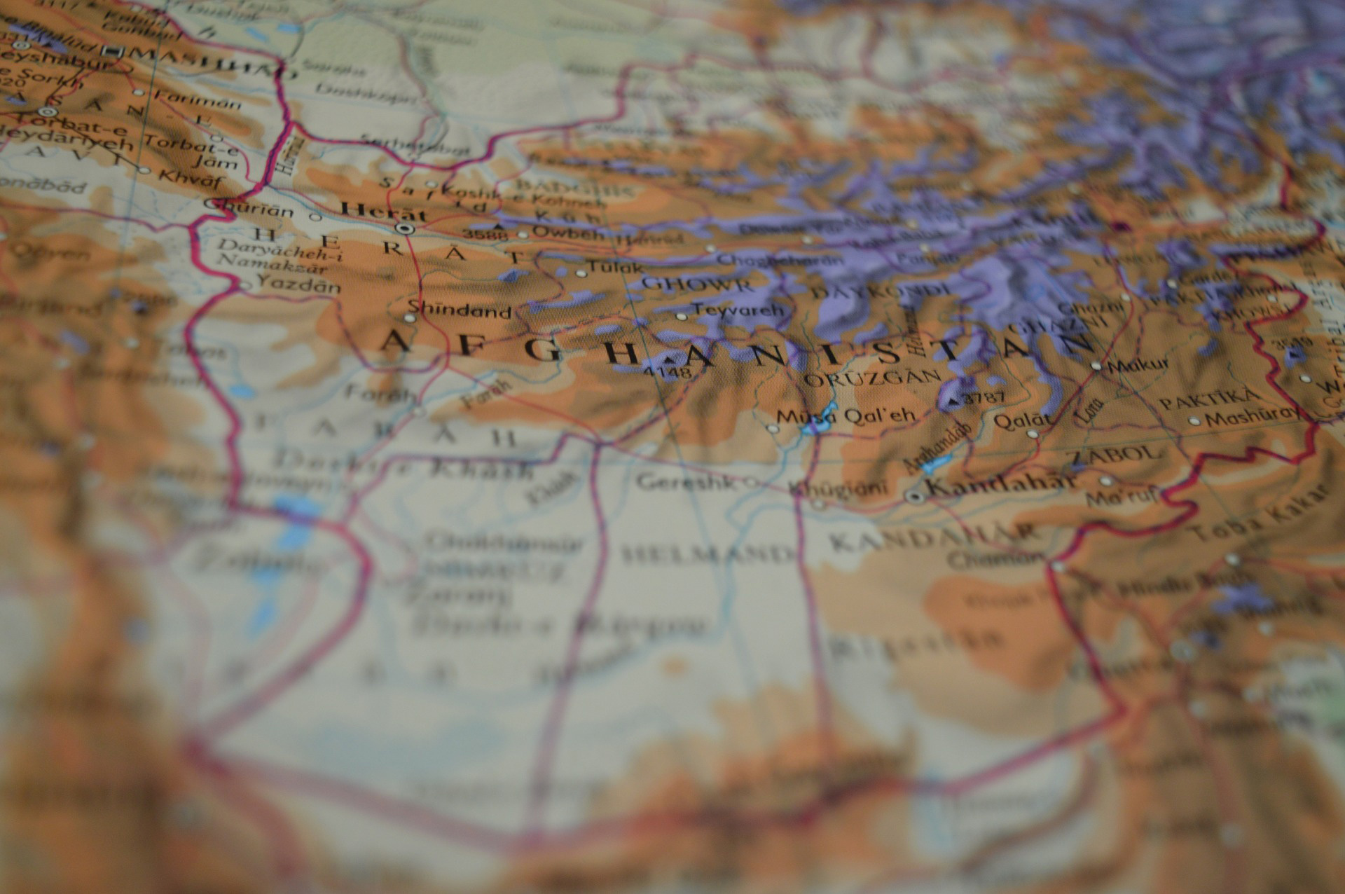
- The boundary between Pakistan and India is constantly changing. National Geographic can now make each change just once, then move it from its world map to its map of Asia and other products.
Starting in a Common Projection
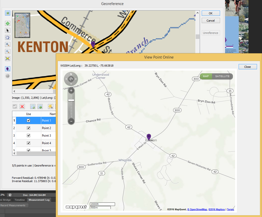
National Geographic starts working on any new map products in MAPublisher. “We want to get off on the right foot, so we make sure that they are all in the common projection from the very beginning,” Lambert explains. His team uses MAPublisher right from the start to georeference files and then to incorporate additional GIS data from federal, state, and county agencies into them. “For example,” Lambert says, “if we get a data set from the National Park Service, we are able to quickly import it and split it into the different layers and styles throughout our entire map series. We can see which trails might be hiking trails, horse trails, or mountain biking trails and quickly apply our styles. We also receive information from the U.S. Geological Survey, such as national hydrological data sets.”
MAPublisher allows users to work in a GIS environment from inside Adobe Illustrator. For example, they can bring in a transportation data set from a county, then click on a road in Adobe Illustrator and bring up a MAPublisher viewing panel to display its attributes, such as its name, whether it is paved, and, if it is not, its clearance. “We can see all the information that these agencies are assigning to these different lines,” Lambert says. “Adobe Illustrator and MAPublisher work together seamlessly.” By contrast, he points out, with other programs you have to exit one and go into the other.
Reconciling Conflicting Data
Most of Patterson’s work revolves around making those very familiar black-banded brochures that visitors receive when they enter a national park. He began using MAPublisher in the mid-1990s, when Avenza introduced version 1.0. “We had just started converting our maps from manual production to digital production using Adobe Illustrator as our primary drawing software,” he recalls. “Soon afterward, geospatial data started becoming more available and the quality greatly improved. Of course, we wanted some means to bring these data into the graphic environment of Adobe Illustrator. MAPublisher provided us with the ideal tool for doing just that.”
Early on, Patterson’s team only used MAPublisher to import geospatial vector data into Adobe Illustrator to produce non-georeferenced maps. As the years went by, however, it saw the value of creating entirely geo-referenced maps.
To create a new map of a national park, Patterson’s team begins with an Adobe Illustrator template that contains all of the map layers that it would use for a typical NPS map—including lines, area colors, symbols, and labels. For even greater efficiency, it employs targeted layers with graphical styles applied to them. “A big part of our process at the beginning,” he explains, “is going on an online digital scavenger hunt, essentially finding whatever data we can that is in the public domain, from which we can compile our maps. We then import these various geospatial data sets into the Adobe Illustrator environment with MAPublisher.”
“The most time consuming aspect of map production is reconciling conflicting data,” says Patterson. “For example, analyzing and fixing different road data sources that don’t match with one another is an arduous process. However, thanks to the data manipulation tools in MAPublisher—which allows us to select, sort, and manipulate data by attribute—this task is now much easier.”
Patterson’s team updates NPS maps every year or two or three, depending on each park’s popularity. Working with a geographically-aware MAPublisher document allows it to take the previous printing of its map and import new data into it, which then drops into place where it should. For example, if a park builds a new trail, the park GIS specialist will send Patterson’s team a shapefile for that trail that it can quickly and easily import using MAPublisher. “It just works seamlessly,” says Patterson. Additionally, almost all NPS maps have shade relief art in the background. “We generate the shaded relief and then manipulate it using Avenza’s Geographic Imager tool in Adobe Photoshop. The result is a geographically aware Photoshop file of the shaded relief, which MAPublisher will automatically register to map line work in Adobe Illustrator.”
Geospatial PDFs
Another very important feature of Avenza’s software, Patterson says, is that it enables his team to save all of its printed maps as electronic files in geospatial PDF format for dissemination via the Avenza Maps app and accompanying digital map store direct to digital devices such as smart phones and tablets. Park visitors can then download and use these maps on their location-enabled mobile devices and, because the maps are geospatially aware, a little blue dot will show their location at all times as they explore a park, even in the absence of a cellular data connection.
Before publishing a new map of a national park, Patterson’s team typically field checks it, saved as a geospatial PDF, using the Avenza Maps app on an iPhone. “We refer to this draft map as we canvas the park,” Patterson says. “We can take notes right in the Avenza Maps app, drop locator pins, and record tracks. When finished field checking, we e-mail the data to ourselves and import it into the working map file through MAPublisher. The notes and tracks that we recorded in the field are used to update the final map, improving accuracy.”
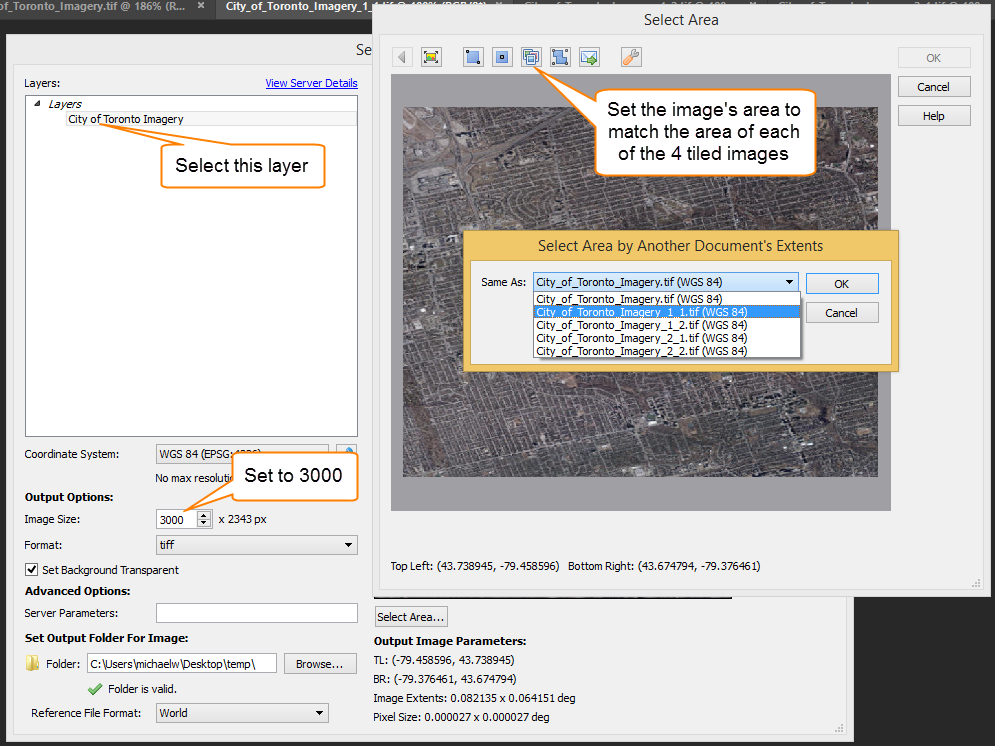
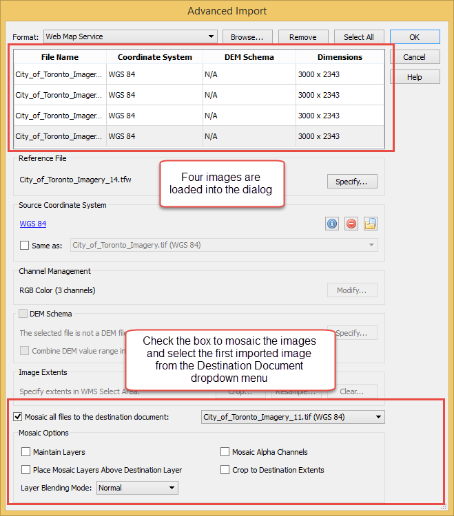
One goal of Patterson’s team is to increase online access to NPS maps. “We are pretty excited about some of the new capabilities in MAPublisher,” says Patterson, “particularly, saving our park maps as Web tiles. We are going through a multi-year transformation right now, converting our maps from the UTM coordinate system to the Web Mercator coordinate system for compatibility with Google Maps, Bing Maps, and Apple Maps. We do all of this through the ‘Export Document to Web Tiles’ feature in MAPublisher, which is really pretty cool.”
Patterson’s team also recently began experimenting with MAPublisher’s Map Web Author tool, which allows quick and easy creation of data-rich and interactive HTML5 web maps from GIS data. It produced a prototype for Harpers Ferry National Historical Park that contains layered information and the ability to explore the map interactively. For example, it allows park visitors to compare contemporary photographs to those taken during the Civil War era at various viewpoints throughout the park.
Other Specialized Illustrator Plugins
There are dozens of plugins that extend Illustrator’s capabilities, for example to edit vector data, concatenate multiple paths, or precisely position nearby objects. Here is one list of Illustrator plugins. CADtools and VectorScribe are particularly noteworthy in this context, because they show that a professional base of CAD users like Illustrator as their working environment, just as GIS and mapping professionals do.
HotDoor’s CADtools 10 plugin provides an extensive set of CAD capabilities—including drawing, editing, labeling, dimensioning, transformation, creation, and utility tools—inside Illustrator. For example, users can insert dimensions or labels on objects, paths, or points in space, which update in real time in response to changes in the artwork. The can also move, transform, and measure objects with precision.
VectorScribe enables users to reduce file sizes by eliminating excess points while maintaining the shape of paths; slide points along paths, extends paths, or trim them; accomplish complex vector editing, such as adding points to tangencies, reverse paths, or smoothly connect curves to straight lines; edit corners on dynamic shapes; or dynamically measure distances and areas along paths.
Conclusions
The sources of geospatial data now include unmanned aerial vehicles (UAS), the Internet of Things (IOT), and myriad consumer devices and, consequently, the amount of available geospatial data is growing exponentially. At the same time, professionals and consumers now expect location to be routinely embedded in everything they do on their digital devices. MAPublisher helps cartographers keep up with this accelerating cycle of supply and demand by making it easier and faster for them to make beautiful maps. Recent attempts by other GIS software vendors to address the increasing demand for cartography and map creation within the Adobe environment is evidence that making maps in Adobe Illustrator is the preferred way to go. With MAPublisher leading the way, it is a workflow that is here to stay.