My Account     Contact Us     Cart

Map-making for the #30DayMapChallenge: Day 4 – Hexagons

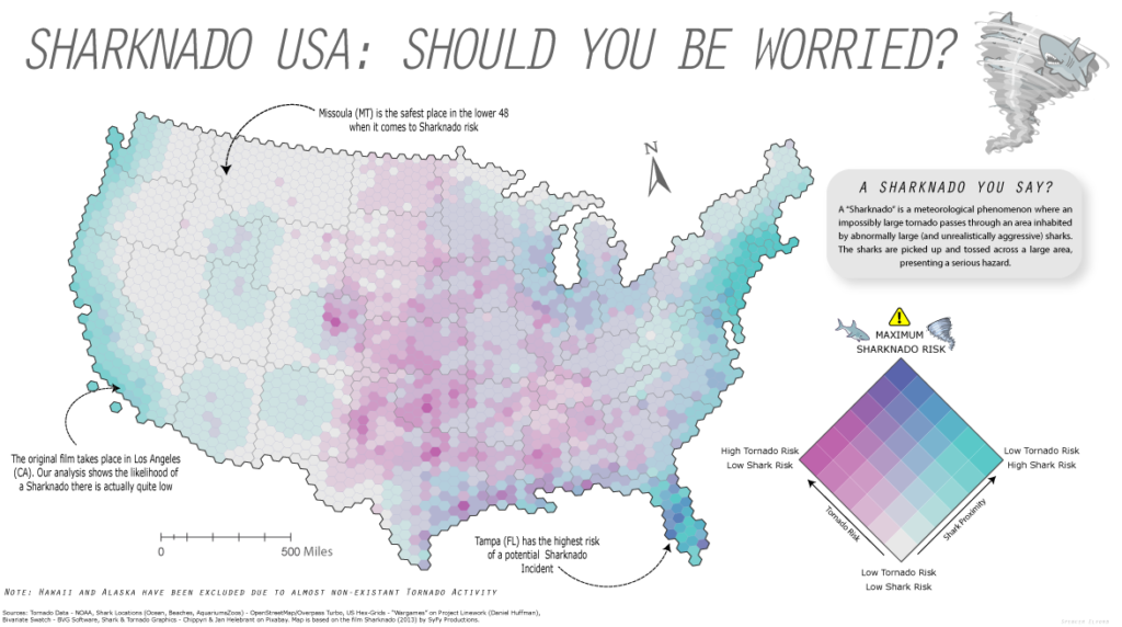
Yesterday was Day 4 of the #30DayMapChallenge, with the goal being to create a map using “Hexagons”. In the spirit of the challenge, we took a not-so-serious approach to create a fun map of “Sharknado Risk” based on the 2013 film “Sharknado” using MAPublisher tools and a really neat hexbin dataset for the United States. This map was in part created for NACIS 2021, and you can see how we created the map by watching the full video presentation included below. This blog also includes a few supplementary notes if you wish to follow along.

What exactly is a Sharknado?

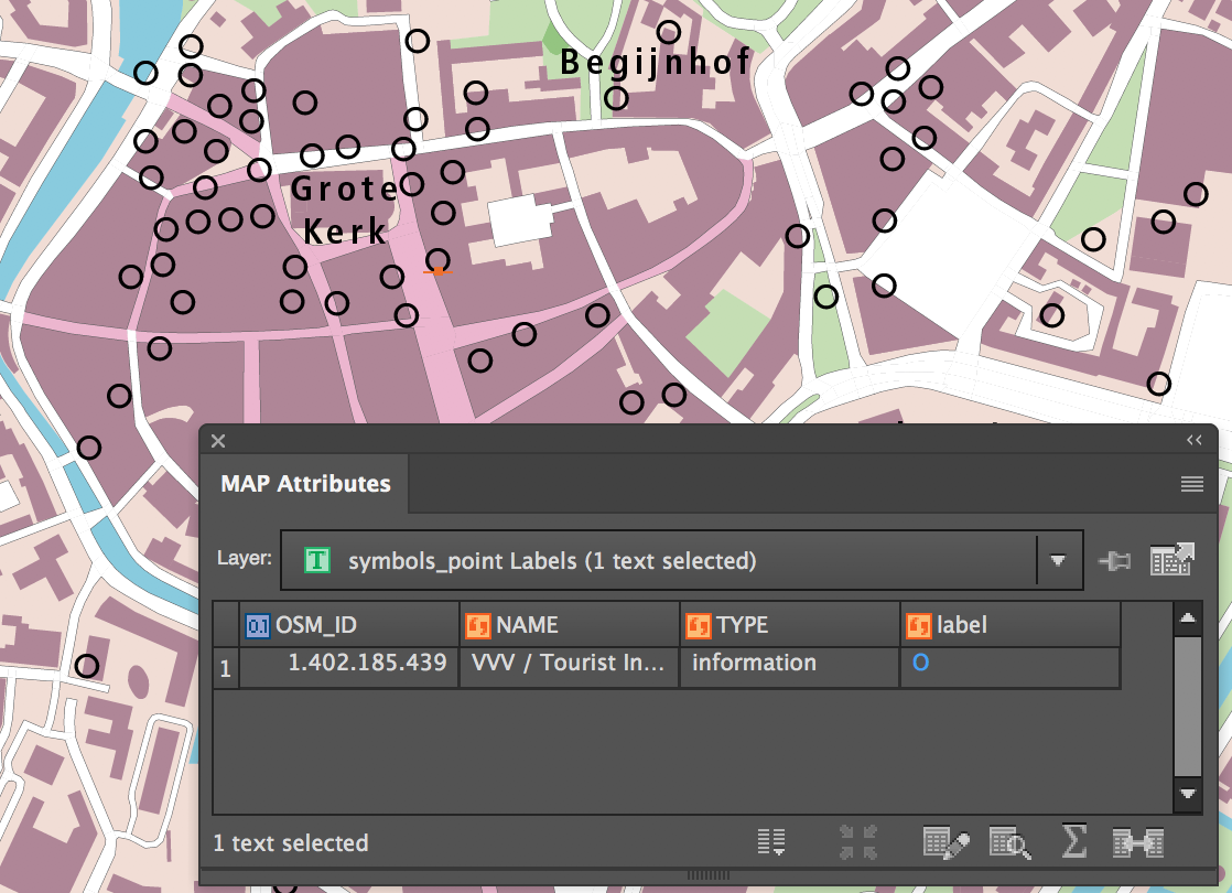
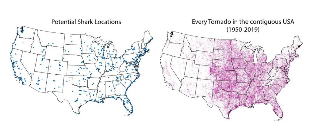
A sharknado is a fictional meteorological phenomenon that occurs when a large tornado scoops up some sharks, transports them some distance, and finally disperses across a populated area. Generally speaking, if a given area is close to potential shark habitats (be it an aquarium, a zoo, or even the ocean) and has a high frequency of tornadoes, the area is more “at-risk” of experiencing a sharknado. To that end, we gathered some great open datasets to help us map this risk. We collected a shapefile documenting point locations for every single tornado in the country dating back to 1950. With this dataset, we can determine the relative frequency of tornadoes for a given area. From OpenStreetMap, we estimated potential locations for sharks by collecting point coordinates for every aquarium, marine park, aquatic zoo, and ocean-facing beach. We used Overpass Turbo to query and extract these points to a spatial dataset and imported them into Illustrator using MAPublisher. Check out this great tutorial (produced by Steve Spindler!) that covers techniques for importing Overpass Turbo data into MAPublisher. The tutorial was part of our ongoing Mapping Class series, a video-focused series that provides helpful tips, techniques, and workflows from real-world cartographers.

Aggregate data with Spatial Join

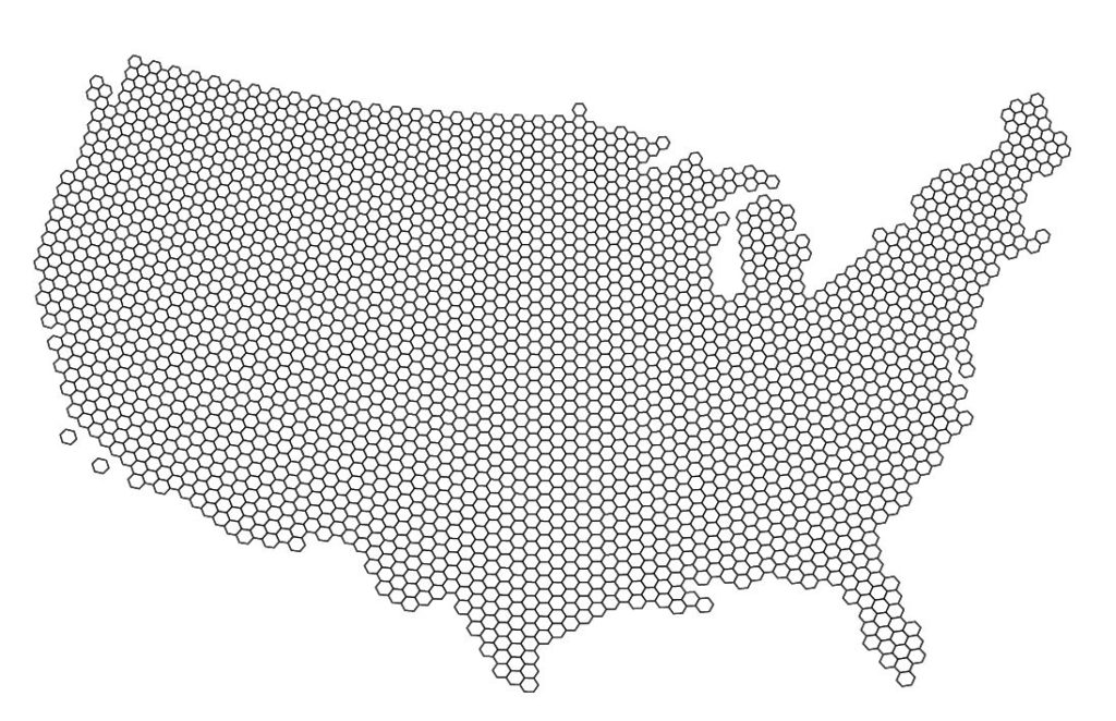
Since the challenge of the day is hexagons, we needed a way to get our messy point data into our clean “hexbin” format. The Spatial Join tool allows us to aggregate our point data (Tornado and Shark Locations) into a single hex-grid polygon dataset.

Credits to Daniel Huffman’s projectlinework.org for making this dataset available!

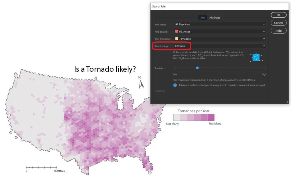
The Spatial Join tool includes several different options for “spatial relationships” that will determine how our point data is joined to the new hex-grid. We can also specify how the tool will aggregate the attribute information for our joined data. In this case, we join our Tornado point data based on a “contains”  spatial relationship. This will aggregate all tornado points that are “contained” within a given hexbin. We also specify that the tool should aggregate the attribute information for all “contained” tornados by tallying up the number of tornado points within each hex. Since we know the dataset spans a 69-yr period, we can easily calculate the average annual tornado frequency for each hexagon.

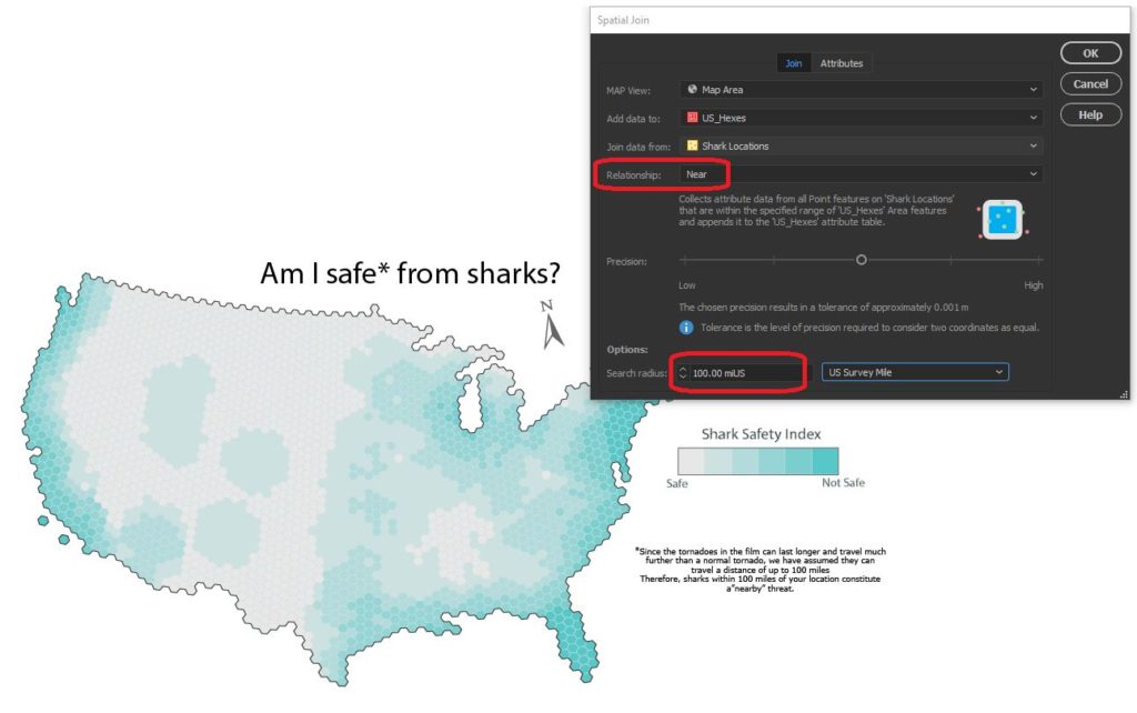
We apply a similar technique to our shark location data, this time specifying a “near” spatial relationship. We used some back-of-the-envelope math to estimate that a Sharknado (as it appears in the film) lasts substantially longer and travels farther than a normal tornado, meaning sharks as far away as 150 miles still present a potential risk. We can specify a search range of 150 miles and this will be applied to our spatial relationship as a cut-off distance. 


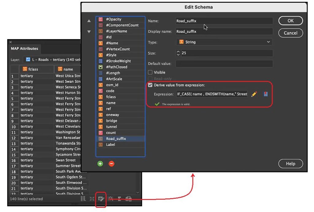
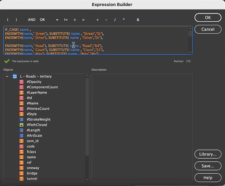
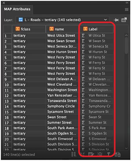
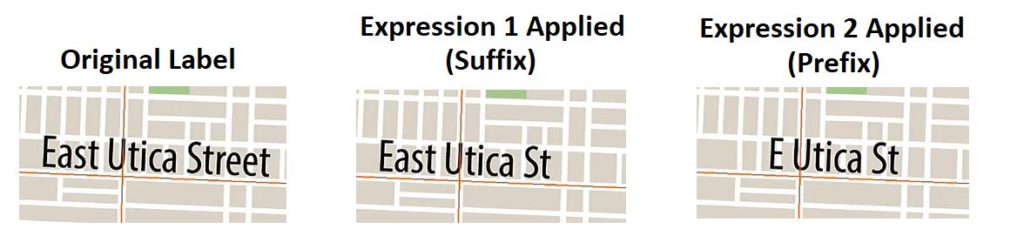
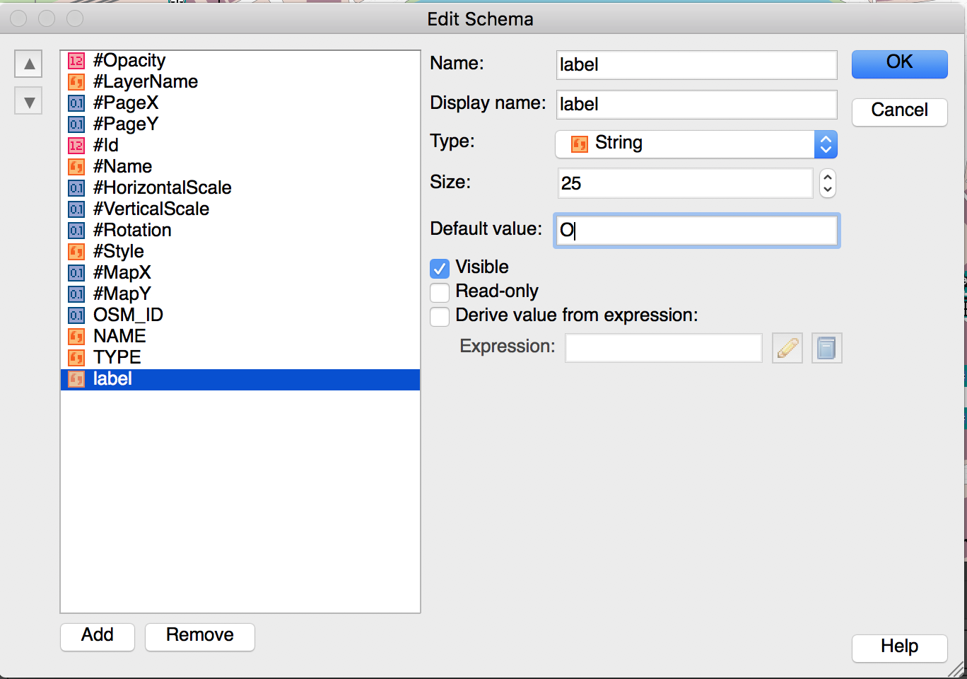
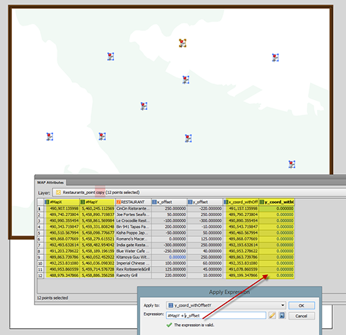
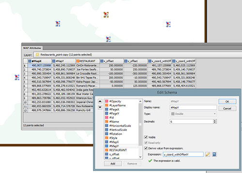
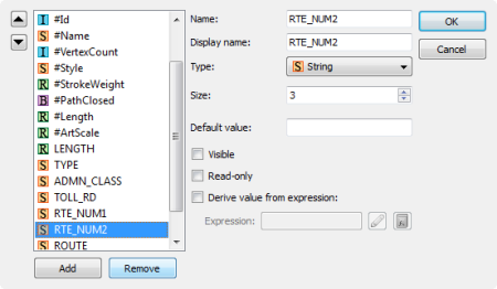
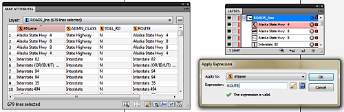
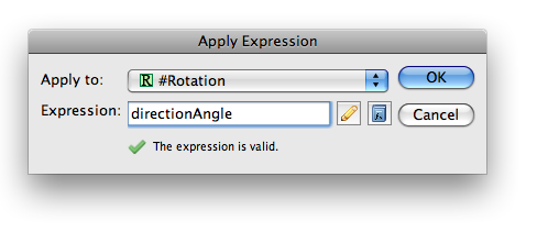
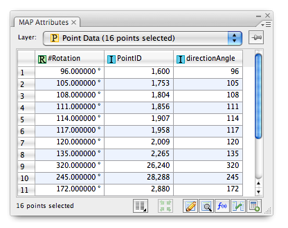
Edit attributes with expressions

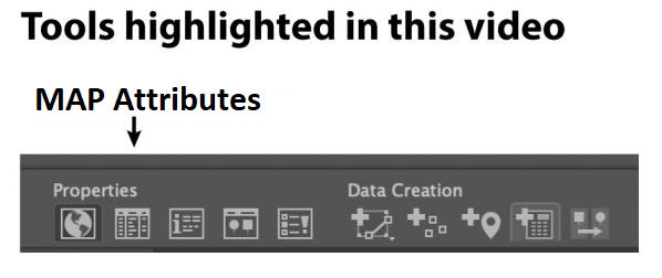
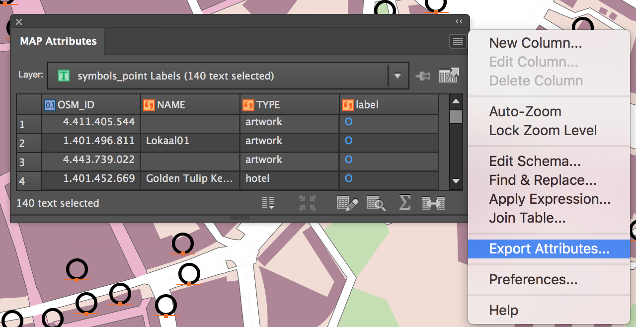
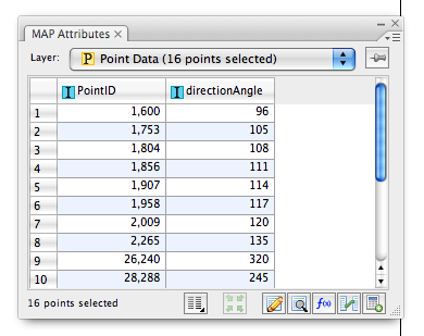
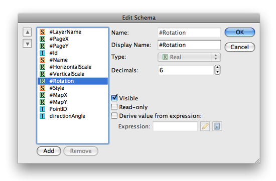
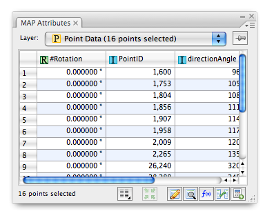
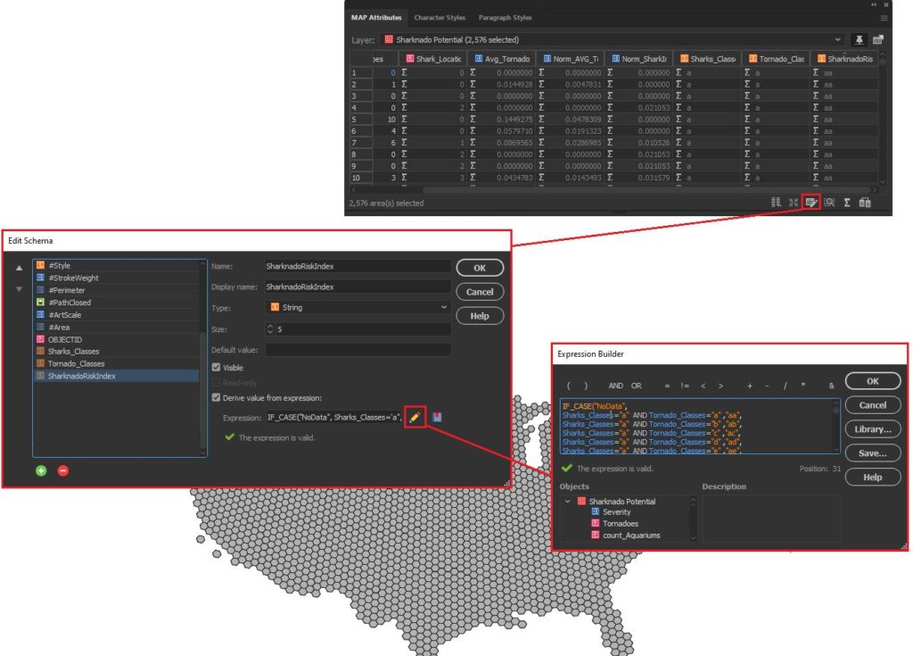
We assumed that Sharknado risk is highest when a given area is prone to tornadoes and also has a high concentration of potential shark locations. Given this, we came up with a basic equally-weighted, bi-variate risk index to assign a “Sharknado Risk” score based on these two variables. To calculate this score for each hexagon in our hexbin grid, we applied some custom expressions using MAP Attributes. First, we assigned a Tornado risk score from 1 to 6 based on the low to high frequency of tornadoes. We assigned a similar score for “Shark proximity” based on the concentration of potential shark locations. Finally, we combined these values into 36 unique scores to evaluate sharknado risk.

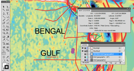
Stylize maps easily with MAP Themes

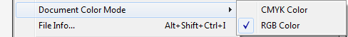
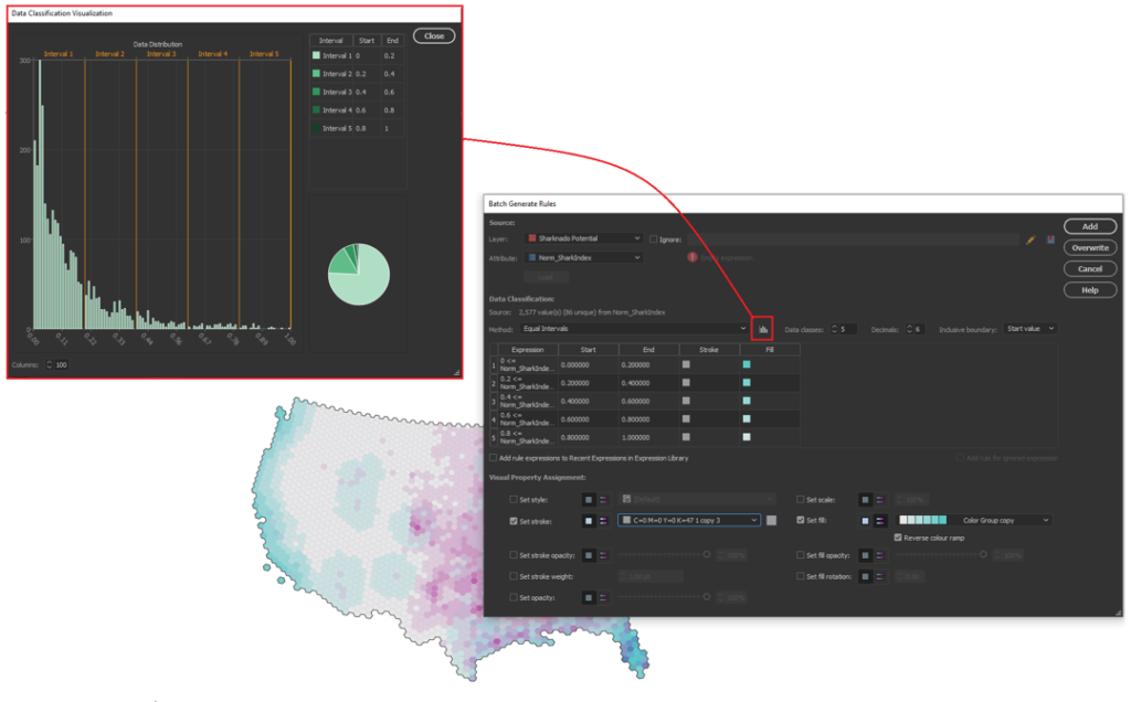
The final step is to stylize our map and create a layout. With MAP Themes, we can create rules-based stylesheets to easily stylize our map data in no time. MAPublisher comes with a great selection of built-in MAP Swatches, including several color brewer-based swatches that work great for choropleth-style maps like this. We used these swatches to create a custom, bi-variate swatch group to visualize each score of our “Sharknado Risk Index”. The MAP Themes tool also provided a neat data distribution viewer, which also allows us to inspect a histogram of our dataset. Although we used discrete categories for each of our risk scores, the data distribution viewer is very useful when working with continuous datasets since it allows you to see how your bin-widths will affect the display of colour on your choropleth.
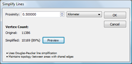
The final touches

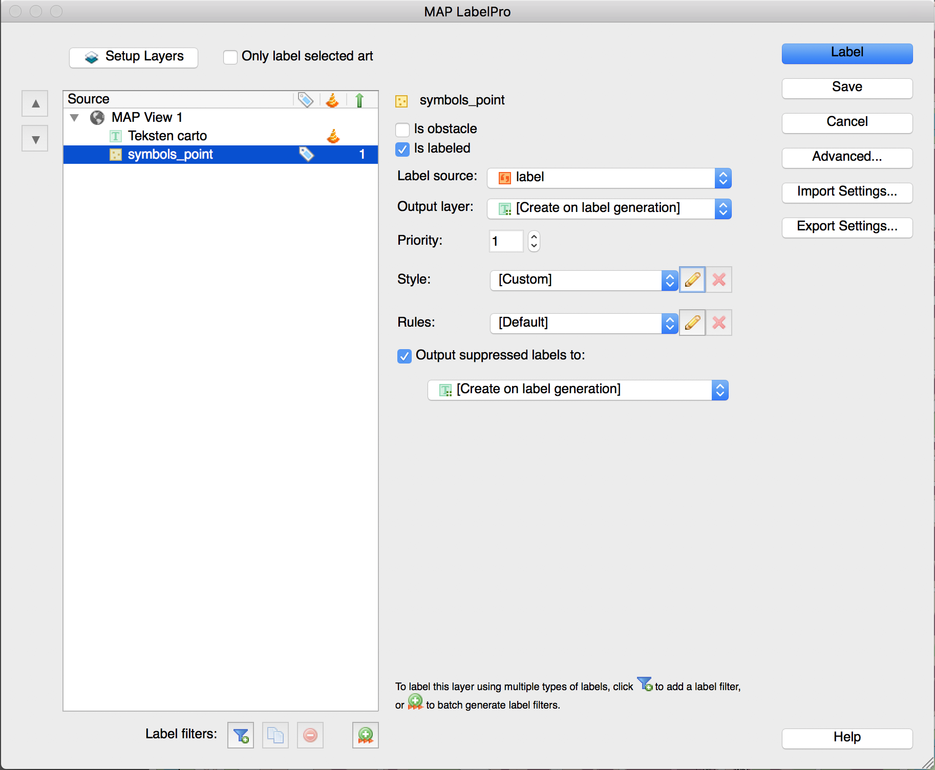
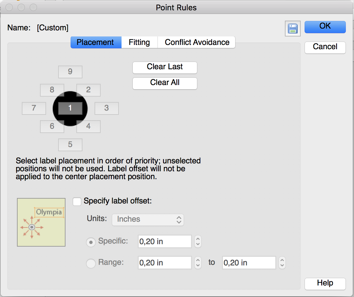
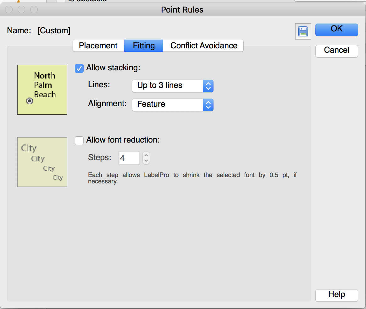
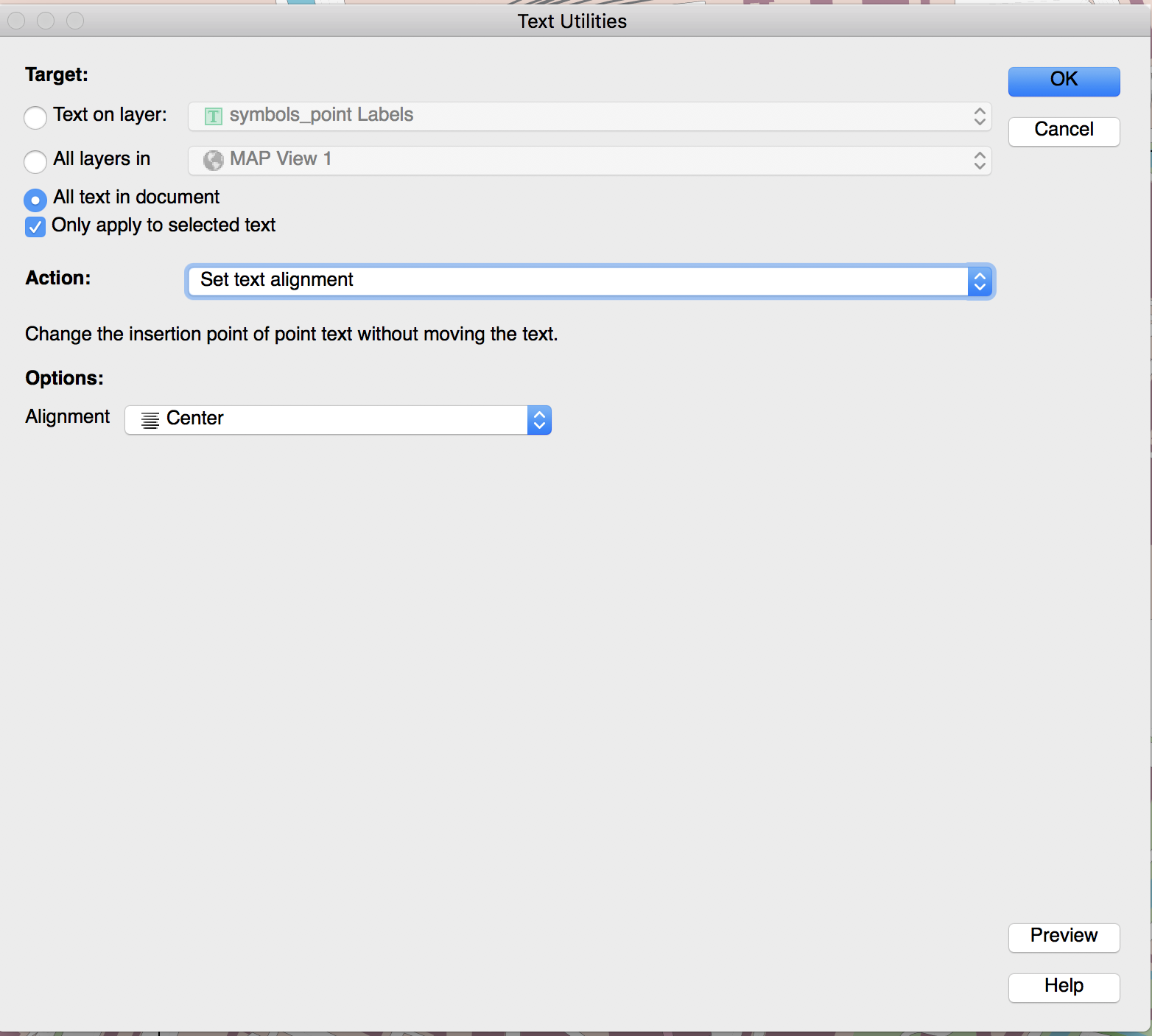
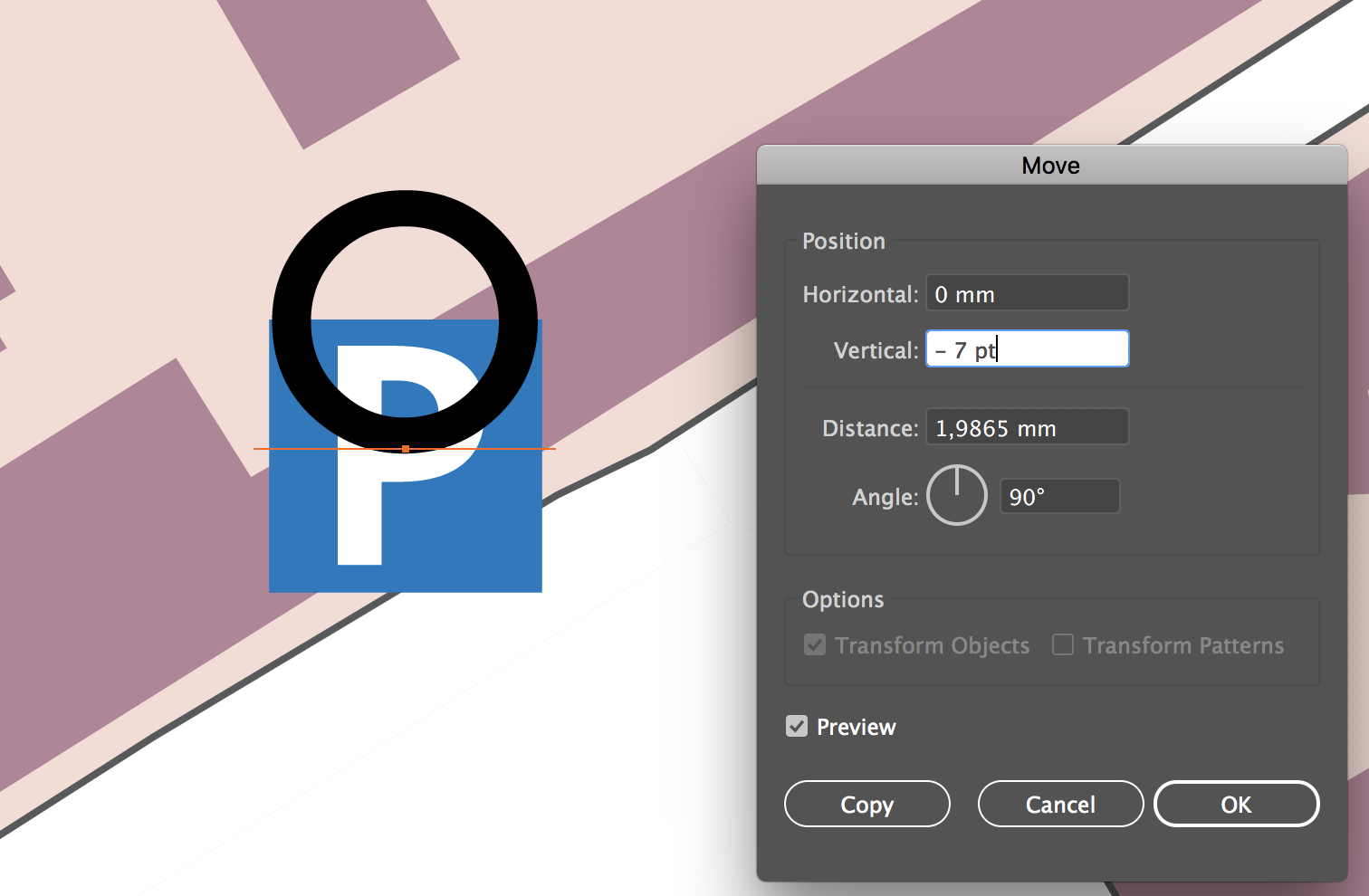
With stylization complete, Day 4 of the #30DayMapChallenge is almost in the bag. We can create a north arrow, and a scale bar and create a custom legend to facilitate easy interpretation. Since we are still within an Illustrator environment, we can use all the powerful native illustrator tools to add graphical design elements, text, and artwork to create a fun, infographic-style map. Although we were happy to call the map finished at this point, the great thing about making maps is there is also room to add more. For example, we might try using LabelPro to create custom labels that mark high and low-risk areas, or we could create insets to highlight specific regions of interest. The possibilities are endless!

We had a great time putting together this fun map for the #30DayMapChallenge, and we are excited to see what we can do for the remaining themes on the calendar! For those of you who are also making maps for the challenge, a reminder that the Avenza Map Competition is still accepting submissions. Share your map, compete with other map-makers in the community, and win some great prizes!

See a PDF version of the map here.

Mapping Class: Efficient Labeling using attribute expression builder with Steve Spindler

Welcome back to this month’s edition of Mapping Class. The Mapping Class tutorial series curates video tutorials and workflows created by experienced cartographers and Avenza software users. Joining us once again is Steve Spindler, a longtime MAPublisher user, and expert cartographer. Steve is here to show you a quick tip for using the attribute expression builder within MAPublisher to quickly perform batch edits of labels. 

Steve has produced a short video to demonstrate how he uses the expression builder to quickly edit street names. The Avenza team has produced video notes (below) to help you follow along.

***

Label efficiently using Attribute Expression Builder
by Steve Spindler (video notes by the Avenza team)

With MAPublisher, labeling your maps is a breeze. With powerful tools such as LabelPro, labeling is only a matter of selecting the data you want to label, and configuring a robust set of rules that control how each label is placed and styled. But before you can start labeling, you must have high-quality, accurate attribute information for your map data. Since labels are typically generated by displaying text values contained in an attribute column, it is important that attributes are not only accurate but are also formatted in a way that is optimized for display on a map. In many cases, cartographers need to spend time reformatting or editing attribute information before they can generate labels, a process that can become quite time-consuming. Nowhere else is this problem more common than when dealing with street names and road network data.

This image has an empty alt attribute; its file name is Tools.jpg

When labeling streets, cartographers often spend time correcting, or even generating brand new attribute information that can be used to create more concise, effective street labels. This typically involves changing street prefixes and suffixes to a condensed short form (i.e “North Cherry Boulevard” becomes “N Cherry Blvd”). For smaller projects, this can be done by manually editing the individual attribute values directly within the MAP Attribute panel. For large projects, especially those dealing with hundreds or even thousands of map features, manual editing would be very time-consuming.

For a more efficient approach, Steve shows how you can use the Expression Builder to easily modify large selections of attribute values. The first step is to open the MAP attribute table, which displays all the attribute information contained within a specific map layer. Steve identifies the attribute column that contains the text street names and will use this to build out a new attribute column to create his labels.

This image has an empty alt attribute; its file name is Buiiklder-1024x691.jpg

Next, Steve opens the Edit Schema window of the attribute table. Here, you can access column information such as the data type, default value, field visibility, and most importantly; the expression builder.

The expression builder may seem intimidating at first, but with a little bit of effort, it can be an incredibly powerful tool for calculating attribute values and performing batch-edits on your data. The tool uses built-in operators and items in the objects list (attribute names and values, constants, functions) to calculate custom attribute information based on a specified set of expressions. In this case, Steve first creates an expression set that modifies the suffix values in the Street name field (i.e “Boulevard”) and substitutes them with the appropriate short form (“Blvd”). The expression is used to populate a new attribute column called “Road_suffix”. The end result means attribute values such as “East Utica Street” will be passed to a new attribute value of “East Utica St”.

This image has an empty alt attribute; its file name is inputs.jpg
IF_CASE(name,
ENDSWITH(name, “ Street“),SUBSTITUTE( name , “Street”, “St”),
ENDSWITH(name, “ Drive“),SUBSTITUTE( name , “Drive”, “Dr”),
ENDSWITH(name, “ Road“),SUBSTITUTE( name , “Road”, “Rd”),
ENDSWITH(name, “ Court“),SUBSTITUTE( name , “Court”, “Ct”),
ENDSWITH(name, “ Way“),SUBSTITUTE( name , “Way”, “Wy”),
ENDSWITH(name, “ Lane“),SUBSTITUTE( name , “Lane”, “La”),
ENDSWITH(name, “ Route“),SUBSTITUTE( name , “Route”, “Rt”),
ENDSWITH(name, “ Boulevard“),SUBSTITUTE( name , “Boulevard”, “Blvd”),
ENDSWITH(name, “ Turnpike“),SUBSTITUTE( name , “Turnpike”, “Tpke”),
ENDSWITH(name, “ Avenue“),SUBSTITUTE( name , “Avenue”, “Ave”),
ENDSWITH(name, “ Place“),SUBSTITUTE( name , “Place”, “Pl”),
ENDSWITH(name, “ Circle“),SUBSTITUTE( name , “Court”, “Cr”),
ENDSWITH(name, “ Highway“),SUBSTITUTE( name , “Highway”, “Hwy”),
ENDSWITH(name, “ Expressway“),SUBSTITUTE( name , “Expressway”, “Exp”)
)


Next, Steve creates a second set of expressions that will further adjust his Road_suffix attribute column to substitute any street name prefixes (North, East, South, West) with their corresponding short-form (N, E, S, W). This second expression (see code block below) is used to populate another new attribute column called “Label”, which will ultimately be used to generate the final formatted label layer. 

((IF_CASE( Road_suffix ,
STARTSWITH(Road_suffix, “West “), SUBSTITUTE( Road_suffix, “West “, “W “),
STARTSWITH(Road_suffix, “South “), SUBSTITUTE( Road_suffix, South “, “S “),
STARTSWITH(Road_suffix, “North “), SUBSTITUTE( Road_suffix, “North “, “N “),
STARTSWITH(Road_suffix, “East “), SUBSTITUTE( Road_suffix, “East “, “E “)
))

This image has an empty alt attribute; its file name is ExpressionAttributes.jpg

Note that these expressions are specific to the dataset and map area Steve is using for his project. When using expression builders for your own maps, pay careful attention to the attribute values specific to your area of interest. The best part about expression sets is that they are highly flexible, meaning you can build upon and modify existing expressions, save them to your library, and even use them across multiple different mapping projects!

With his newly created “Label” attribute column, it’s simply a matter of configuring the LabelPro tool to display these formatted label values. With a bit of configuration, the end result is a clean, uncluttered, collision-free label layer. The labels now use all the correct prefixes and suffixes Steve required. By saving his expression sets to his library folder, Steve can now quickly and easily repeat the exact same batch-editing process for new maps with only a few clicks! 

This image has an empty alt attribute; its file name is ExpressionBuilder-1024x249.jpg

***

About the Author

Steve Spindler has been designing compelling cartographic pieces for over 20 years. His company, Steve Spindler Cartography, has developed map products for governments, city planning organizations, and non-profits from across the country. He also manages wikimapping.com, a public engagement tool that allows city planners to connect and receive input from their community using maps. To learn more about Steve Spindler’s spectacular cartography work, visit his personal website. To view Steve’s other mapping demonstrations, visit cartographyclass.com

Optimizing Point Symbol Placement with MAPublisher LabelPro

This post was contributed by Hans van der Maarel of Red Geographics.


The problem with using GIS data for point symbols is that depending on the scale and symbolization you often end up with symbols partly overlapping each other. Of course, the symbols can be manually moved around after initial placement to get a more aesthetically pleasing result, but that can be a tedious and time-intensive task.

Thankfully, there is a way to automate at least part of this process by using MAPublisher and LabelPro.

Example map of Breda, The Netherlands

This example shows the heart of an old European city (Breda in The Netherlands to be exact). The map is composed of Dutch Top10NL topographic base data, a few labels were manually added for larger features (such as the park), and points imported from OpenStreetMap (OSM) and styled using a Map Theme. As you can see, there are a number of spots where the symbols are densely located and overlap each other.

The MAPublisher LabelPro add-on is capable of collision-avoidance to make sure overlaps don’t happen. But it only works when generating labels (text). Fortunately, the solution is to trick LabelPro into processing symbols too, so that they can benefit from better placement without overlaps.

Let’s start by adding a column to the attributes to the OSM points layer and filling it with a default value, a capital O.

Thankfully, there is a way to automate at least part of this process by using MAPublisher and LabelPro.

Editing the attribute schema

Next, determine how big the symbols are. On the artboard, use the Type tool to place a capital O and adjust its size so that it’s about the same size as one of the point symbols. In this case, a 14 pt Futura Medium, shown here in red, seems to cover it well (your results might be different).

Determine the approximate font size

Futura is a good font in this case because the O is a perfect circle. Once you’ve determined the approximate font size to use, delete the O text as it won’t be needed anymore.

Next, set up the LabelPro labelling rules. Since there is already a layer with the manually placed labels and the symbols shouldn’t interfere with them, the manually placed labels will be designated as an obstacle layer. The symbols layer will be labelled with the attribute created earlier and the style set to the font and size that was just determined.

Set obstacle layer

Setting the appropriate rules partly depends on personal preference but it’s important to specify that the placement prefers the center position (position 1 on the placement control). In other words: if there’s enough space for placement, the label doesn’t need to be moved or offset. Another important rule to configure is that font reduction should be turned off. All of the labels (eventually symbols) are going to be a fixed and similar size.

Set placement point rules
Set fitting point rules

Also, another good practice is to specify a suppression layer. Any labels that can’t be placed with the rules set will be placed on the suppression layer. After placement, you can determine if any labels need to be adjusted manually.

Let’s label! Go ahead and label with these settings and afterward hide the original symbols layer and the suppression layer. The map is filled with O’s where the original symbols are located.

O labels placed

At first glance, this does not seem very useful, but closer inspection shows that the labels have retained the attributes of the original OSM point symbols.

Attributes migrated to the O labels

This means that if they can be turned back into points, they will be able to be styled!

In order to turn them back into points, a text reference point needs to be created. In other words: a little dot on the text selection line, in the center of the O. This is a two-step process. First, select all the O’s on the artboard, open MAPublisher Text Utilities, and set the Action to Set text alignment and Alignment to Center. This action changes the alignment of the text without changing the actual position of the text (due to LabelPro labeling the text alignment is different based on where the label ended up in relation to the original point). This step takes care of the horizontal positioning.

Set text alignment in MAPublisher Text Utilities

The second step is to adjust vertical positioning. Vertical positioning is adjusted by moving all text up by a certain distance. Make sure all the O’s are selected, then use the (Adobe Illustrator) Move tool. In the Position group, set the Horizontal to 0 (no adjustment here since Text Utilities was used), set the Vertical to minus half the text size (font size in this example was 14 pt, so a vertical adjustment of -7 pt), and the Angle to 90 degrees.

Use the Move panel to fine tune position

For reference, this example is zoomed into a symbol that did not get displaced.

Next, these labels need to be turned into point symbols. There is a handy option in MAPublisher Text Utilities that can do that, but it places a point to the lower left of the text and the symbols need to use the center text reference point that was just created. Instead, with all of the O labels selected, open the MAP Attributes panel and export the attribute table to a text file. Make sure to specify the option Export All Attributes because there are two important hidden attributes needed to make this work: #MapX and #MapY, which are the coordinates of the text reference point.

Export attributes to a .txt file
(Click for larger version)
Export attributes to a .txt file

Using MAPublisher Import, add the attributes text file that was just created to the map and make sure to appropriately specify #MapX and #MapY in the X and Y coordinate columns.

Import .txt file as Delimited XY

Since there is no projection information stored in the text file, you’ll need to specify that the coordinates are in the same system as the MAP View it’s coming from and you’ll need to add it to that MAP View upon import.

On the map, there is now a new point layer and because they still have all of their original attributes, the layer can simply be added to the MAP Theme to have all the point symbols reapplied to them instantly. Let’s admire the results:

Symbols reapplied with MAP Themes

If needed, repeat the last few steps for the suppressed labels as well (to a different file and different layer of course) to see what still needs to be done manually.

Placing Text with an Offset Value Using MAP LabelPro

Having introduced some background information about text insertion point coordinate values in a previous post, it would be good to explore if this method works when trying to place text objects (annotations/labels) with a specific offset value. For example, if you have a point layer and there is an attribute for the offset value so that every object has a different offset value.

An Attribute table with the offset value for every object

Placing text objects with a specific offset is possible in MAP LabelPro. You can specify the Label Offset value in the MAP LabelPro dialog box. However, this setting will be applied to all text labels. In the example below (see screenshot), all the text will be placed 0.2 inches away from the object. However, that does not help when every point has different offset value like this example. Also, MAP LabelPro uses page units, not the world/map units. In this example, the offset distance was specified in the world/map unit (metres).

The offset option in The Point Rules dialog window from MAP LabelPro.

There are two methods you can accomplish to make the text placed with offset value. The first method is the same as the step shown above. You can adjust the text placement position by calculating the “ideal” coordinate for the text insertion point. From a MAP layer (point, line, or area), generate text with a MAPublisher feature (MAP LabelPro or Feature Label).  Then adjust the text position (maybe you will have to calculate a new position by adding/subtracting the offset values from the current point), then apply it to #MapX and #MapY. The second method is to adjust the position of the points first before labeling.

In the example below, a point layer with offset values in the attribute: x_Offset and y_Offset.

An example map with offset attributes (x_offset and y_offset)

Step 1: Calculate coordinates with offset.

  1. Create a copy of the layer just because the point value will be adjusted.
  2. Make the #MapX and #MapY visible (so that it’s easy to see when calculating).
  3. Create new columns (here we created “x+coord_withOffsetX” and “y+coord_withOffsetY”).
  4. Calculate the new coordinate of the points for X and Y (here we used Apply Expression) as shown below.

Step 1: Calculating the coordinates with offset

Step 2: Move the points to the calculated coordinates with the offset values.

Use the same method as the one introduced in the previous post. This method works for the Point layer as well. Open the Edit Schema window and apply “x_coord_withOffset” and “y_coord_withOffset” to #MapX and #MapY, respectively.

Step2: moving the points to the calculated coordinates with the offset values

Now, the points are moved to new position. The red point is the original and the blue points are the ones moved to the offset. Now you can label each points. After placing labels for the point layer (blue), you can make the point layer invisible.

The point position is adjusted by #MapX and #MapY

Now you can run the label engine (MAP LabelPro / Label Feature) for the new point layer with offset.

Optimizing Adobe Illustrator Documents with MAPublisher for Geospatial PDF Export

Adobe Illustrator documents with GIS data can be exported to georeferenced PDF files thanks to the MAPublisher Export Geospatial PDF feature. A geospatial PDF is an Adobe Acrobat file that contains geospatial coordinates. With coordinates, users can view and interact with the PDF to find and mark location data. MAPublisher exports all the MAP Attributes data in an Adobe Illustrator document into the geospatial PDF. Attribute values can subsequently be accessed and searched in Acrobat 9 (and 8 with limitations).

In order to ensure the best interoperability and geospatial PDF output results from your MAPublisher documents, the following work practices are recommended:

Convert document color mode to RGB

To ensure predictable color results, it is highly recommended to convert the documents color mode to RGB prior to exporting to Geospatial PDF. This is advisable especially if generating geospatial PDF documents to be used in conjunction with the PDF Maps app for IOS devices. The document color mode can be changed in Adobe Illustrator through File > Document Color Mode > RGB Color.

Colour mode

Crop data to the required extents using the MAP Vector Crop Tool

Remove any extraneous data not required for the geospatial PDF document by cropping the map using the Vector Crop Tool (located in the Adobe Illustrator Toolbar). If necessary, exclude data from being cropped by locking the its the appropriate layers.

Vector crop

Remove unnecessary layers

Delete any map layers that are not required for the final PDF map document. This may include raster layers, hidden layers, and layers that are outside the mapping extent or art board. Not only will this decrease file size, it will also simplify your layers list and improve organization. Delete layers in the MAP Views panel or the Layers panel.

delete selection

Preserve data contained within sublayers

If your document contains map data organized within sublayers it will be necessary to reorganize/move this data to it’s parent layer if you wish to preserve it when converting to and from geospatial PDF. This is necessary because data contained on sublayers are forced into their parent layer by the Adobe Illustrator PDF exporter. Layers are also required for importing a geospatial PDF back into MAPublisher in order to assign a schema.

Remove unused attribute information

Data sets, especially those available through various data portals and government agencies can contain attribute information not suited or required for our mapping need, or perhaps we are only interested in the geometry of the data for representational purposes. In this case it is advisable to delete any attribute information that does not fulfill a purpose as this will unnecessarily increase the resultant file size. Select your data, open the MAP Attributes panel, and click the Edit Schema button. You may delete and organize your attributes using this panel.

Edit attribute schema

Assign MAPublisher attributes to Adobe Illustrator Object names

This recommendation is not necessary but may be useful in some cases. In MAPublisher the #Id attribute column is a unique identifier MAPublisher uses internally to associate attributes with unique pieces of art. By default the art will have a name of “path” or “compound path” however it may be desirable to tag the object with a unique identifier from an existing attribute column for the purposes of making it easier to differentiate art objects within the Acrobat tree list, for example.

To do this we can use the “Apply Expression” option in the MAP Attributes panel. Simply designate the #Name column as the “Apply to” option while entering the name of the attribute column you wish to derive the attributes from as the “Expression”. For example in the screeshot below we are renaming the art objects contained in the #name column with values stoed in the “ROUTE” column with the results being reflected in the artwork listed in Illustrator Layers panel.

Use the Simplify Line Tool

Reduce the number of vertices available in MAP Line and Area layers by using the Simplify Line tool (located on the MAPublisher toolbar). This differs from the Adobe Illustrator Simplify Path tool because it takes into account X and Y coordinates. The proximity value or simplification tolerance is based on the vertical difference between the begin-end line and points off a line, not the distance between anchor points on the line.

Simplify lines

Geospatial PDFs derived from or include images should be generated as 72 DPI

This has particular relevance when dealing with geospatial PDF files, especially those generated with Geographic Imager. When a 200 DPI (dots per inch) georeferenced image is converted to a geospatial PDF, the image will be embedded in the PDF as a 200 DPI image. However, when displayed by PDF viewing applications such as Acrobat or Illustrator it will appear as a 72 DPI image. Due to this, on export, MAPublisher converts the referencing to 72 DPI format since it must be imported back as 72 DPI

Geospatial PDF at 72 DPI

Following the above recommendations should help ease the transition of your MAPublisher documents to and from geospatial PDF.


Changing the Point Angle using Expressions and Attribute Values in MAPublisher

Here we have placed point symbols for a MAP Point layer. However, we want to change the point angle using the Attribute values.

Step 0: my point (not rotated)

Below is the attribute table for the point data shown above. The field directionAngle is the field containing the symbol rotation value. With MAPublisher, it’s possible to assign this value to every symbol in this layer.

step 1: Attribute data

Open the Edit Schema dialog box from the MAP Attribute panel. Find the field called #Rotation from the attribute field list. This #Rotation field is hidden/invisible by default. Click the Visible option to enable it and click OK.

MAP Attributes > Edit Schema

In the MAP Attributes panel, you can see that the #Rotation field shown. The values in this field is 0.00 degree for every point in the layer. We’ll assign the angle value from the directionAngle field to the #Rotation value .

MAP Attributes panel with the #Rotation field displayed

Open the Apply Expression dialog box from the MAP Attributes panel. Enter the column name directionAngle for the Expression and ensure that the value will be applied to the field #Rotation.

MAP Attributes panel > Apply Expression

Every value from the directionAngle field is now inherited by the #Rotation field.

MAP Attributes: Angle value assigned

As a result, the rotation angle is now applied to every point.

Point symbols after the angle values are assigned

The origin of the rotation is at each point’s registration point. With Adobe Illustrator CS4 and earlier, the registration point is set at the centre of the point symbol. With Adobe Illustrator CS5, the registration point can be flexibly placed. This will be discussed with some examples in a later topic. Stay tuned!

News Archive