

Welcome back to another exciting edition of Mapping Class, a video-blog series where we curate tutorials and workflows created by expert cartographers and Avenza power users from around the world. Today we release Part Two of our Georeferencing Techniques tutorial with Hans van der Maarel, owner of Red Geographics. In Part Two, Hans demonstrates some techniques he has developed for working with more challenging georeferencing tasks, including dealing with unknown projection information and working with scanned maps. If you missed Part One, in which Hans covers the basics of Georeferencing in MAPublisher, check it out here.
Hans has produced a jam-packed video walkthrough detailing his georeferencing process. The Avenza team has produced video notes (below) to help you follow along.
***
Georeferencing Techniques Part Two: Working with Scanned Maps
by Hans van der Maarel (video notes by the Avenza team)
As we discussed in last month’s Mapping Class, georeferencing is the process of taking imagery or map data that lacks geographic location information and associating it with specific coordinates on Earth. Previously, Hans showed us how MAPublisher provides a few tools that make georeferencing simple vector map data a painless process (Check out part one here!). Best of all, using the built-in georeferencing tools, this can be done entirely within the Adobe Illustrator environment.
However, what can you do if you are working with historical maps or scanned images that lack spatial referencing or detailed projection information? This can present a challenge for many cartographers, as the projection information is necessary to create an effective cartographic product that will minimize distortion and maximize the spatial accuracy of the final result. To tackle this problem, Hans shares a series of tips and tricks that he uses for working with scanned historical maps. He uses a beautiful historical map of Northwest Africa to demonstrate his approach.
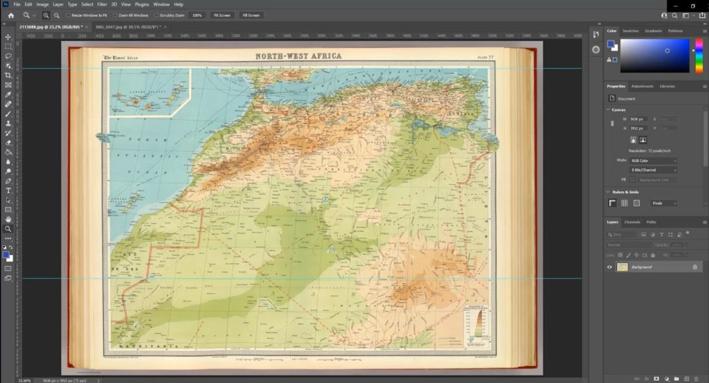
Right away, Hans identifies a few obstacles. First, he notices that the scan is not a perfect copy of the original map. Due to natural curves and bends in the physical paper version of the map, there is minor distortion in the digital image that arose when the map was scanned. This could create problems for georeferencing the image, as the “fitting” process can be susceptible to image distortions, even when a suitable projection is determined. Thus it is always a good idea to examine your scanned map prior to beginning the georeferencing process. Becoming aware of potential issues with the scanned map data can help inform decisions on the data’s suitability for a particular mapping task. Acknowledging that the distortion is relatively minor in this scanned map, Hans chooses to proceed with the georeferencing process.
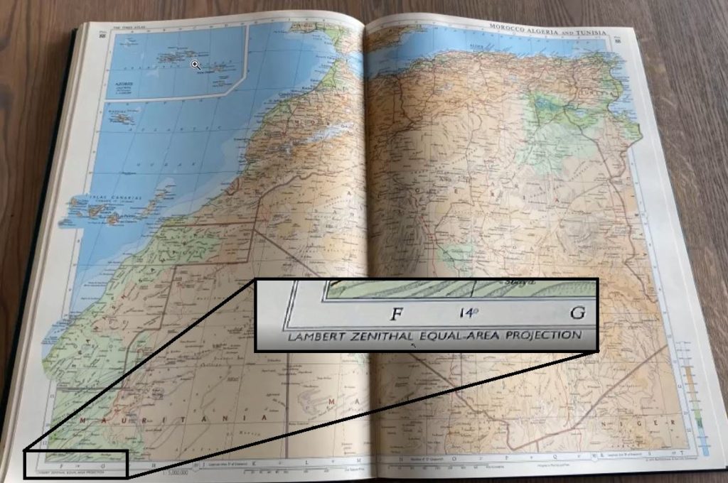
Hans notices that the scanned map image does not provide any details on the original projection information. Instead, Hans must make an “educated guess” on which projection was being used. With a bit of research, he discovers another map from roughly the same era and displaying a similar region. Recognizing the similarities between this map, and his scanned map, Hans decides to implement a Lambert Zenithal (Azimuthal) Equal Area Projection.
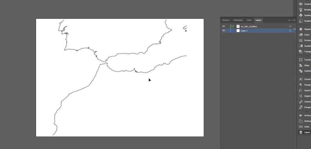
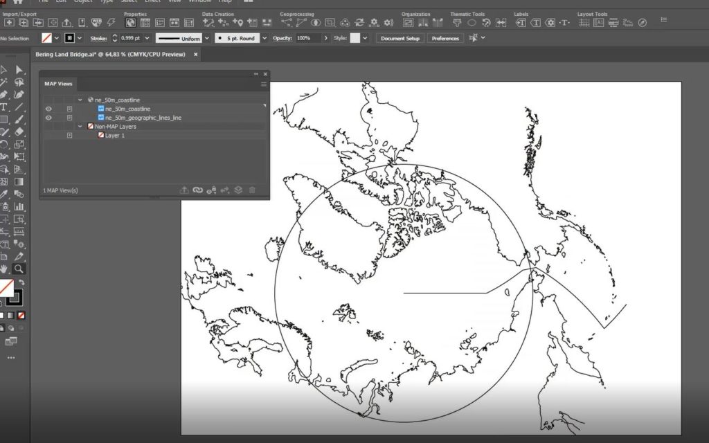
Hans can begin his georeferencing process by first setting up a new MAP View with the Lambert Azimuthal Equal Area Projection, a conical projection used in many atlas-style maps. To help with the georeferencing process, Hans has used the Import tool to display a vector line layer of coastlines using Natural Earth Data. He can use this coastline data as a guide to help align his scanned map during the georeferencing process.
Before moving on, Hans brings up two important things one must consider when working with conical projections: the central meridian and the latitude of origin. When working with scanned maps that include graticule lines, a quick and easy way to help identify the central meridian is to look for the meridian line that closest approximates a straight line. Using the graticules on the scanned map, Hans can approximate a central meridian of about 11 Degrees. In the MAP View Editor, a user can open the projected Coordinate System Editor and modify the definition for the lambert azimuthal equal-area projection to have a central meridian that matches his estimation.

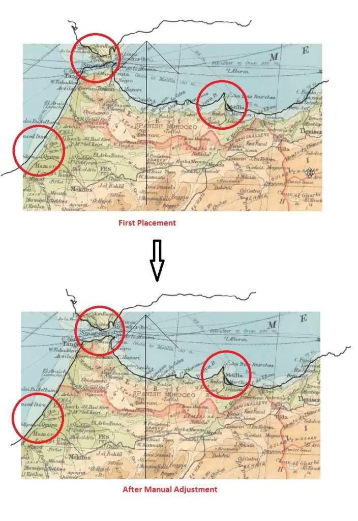
Placing the scanned map layer onto his newly modified MAP view, Hans can then begin the process of manually aligning the map image to match his projected coastline data. One of the easiest ways to support this process is to configure the MAP View editor panel to display layer thumbnails. With this configured, a user can begin manually adjusting the MAP layers until they are suitably aligned.
Hans reiterates that this process is not an exact science. He has made several assumptions on the projection parameters, and the overall accuracy of the original map. He indicates that a user should spend some time trying to get the best possible result, however it will be difficult to achieve a perfect match (especially given the distortions that can occur when a map is scanned from a physical copy). This process can take anywhere from minutes to hours, and requires a lot of manual adjustment, trial and error, and most importantly, patience! The result, however, is that the finalized scanned map layer is correctly projected and georeferenced into a MAP view. From here, adding data layers, annotations, labels, or tracing vector layers from the scanned map can all be completed in a spatially aware mapping environment.
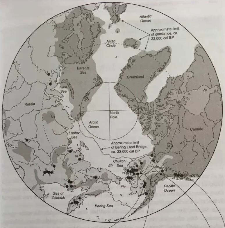
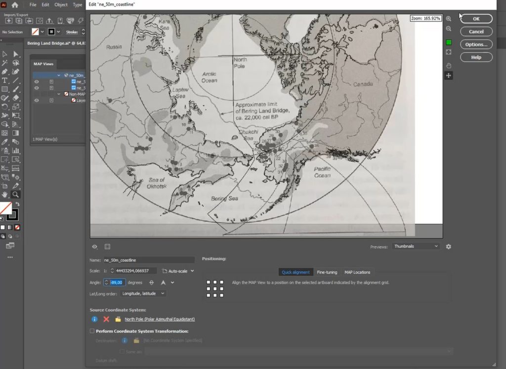
Providing a second example using a slightly different approach, this time Hans uses a map of the Arctic Region. He indicates that although he has been provided with a map of the entire polar region, the client is only interested in the area surrounding the Bering Strait (between Russia and Alaska). As with the previous example, the first step is to identify the best projection to use. Hans correctly guesses that the map provided likely uses the Polar Azimuthal Equidistant Projection based on visual inspection. However, it should be noted that there is room for trial and error here, and users should not be afraid to explore the large coordinate system and projections library included with MAPublisher to try out and test different projections to help narrow down one that fits best.
The first thing Hans notices is that the scanned map image is rotated about -90 Degrees from what is displayed in his reference coastline data. Once again, by visiting the MAP View Editor, Hans can rotate his Map layers without breaking the spatial referencing information of his original map data. By doing this, Hans assures that his map layers are aligned on the same rotational angle, and can then begin to focus on scaling the layers.
Hans uses the MAP view editor panel to apply manual adjustments to the map layers. He notes that a cartographer should always consider the area of the map they are most interested in. For example, although his map covers the entire polar region, Hans indicates the final product will only display the regions surrounding the Bering Strait. Given this, the georeferencing process should be primarily concerned with accurate alignment in the Bering Strait area, while distortion in other areas is seen as acceptable. In the example below, you can see how Hans has achieved a suitable level of georeferencing accuracy in his primary area of interest, despite the non-important areas (i.e the Canadian Polar region, eastern Siberia, Greenland) having relatively low georeferencing accuracy.
With his newly georeferenced scanned map layers. A cartographer can now use the information contained within these scans to supplement a larger cartographic process. For example, Hans can now use the scanned maps to digitize boundaries, or geographic features that may not be present in modern digital datasets (for example, historical boundaries for different countries, or terrain features that are no longer present)
***
About the Author
Hans van der Maarel is the owner of Red Geographics, located in Zevenbergen, Netherlands. Red Geographics is a long-time partner of Avenza and Hans is a well-known power user of both MAPublisher and Geographic Imager. He uses the products for a wide range of cartographic projects for several international organizations and offers training courses and consultancy expertise aimed at developing workflows for clients. In addition to that, he is currently a board member of NACIS. To find out more about Red Geographics, and to see more work by Hans, visit redgeographics.com