My Account     Contact Us     Cart

Articles

Creating a false-color composite image with Geographic Imager for Adobe Photoshop

One of the powerful remote sensing tools available in Adobe Photoshop is to detect the land surface information by creating a false color composite image. Multispectral images contain the reflectance information from the visible and invisible electromagnetic spectrum. Using this information, we can detect many kinds of land surface information. For this example, we will detect the green area using Landsat images imported by Geographic Imager for Adobe Photoshop, which ensures all the georeference information is maintained.

Landsat images consist of several gray scale images, with each image containing one of the bands of the electromagnetic spectrum. For example, in the Geographic Imager tutorial folder, there are a set of Landsat images available. Those gray scale images are from Band 1, 2, 3, 4, 5, 7, and 8.

Landsat Images available in the Geographic Imager tutorial folder

These images need to be combined into one image. The Adobe Photoshop function called “Merge Channels” produces one image by combining mulitple gray scaled images. With this example, those gray scale images from Band 2, 3, and 4 will be merged into one image by assigning a color for each band.

Image analysis trick

1) Open the Landsat image from Band 2, 3, and 4. Note that the Geographic Imager panel shows the information on the coordinate system and image extents.

Georeference information on the Geographic Imager panel

2) Open the Channel panel (Window > Channels). Choose “Merge Channels” from the panel options menu.

Merge Channels

3) In the Merge Channels dialog box, select RGB color as the mode.

Merge Channels - RGB

4) In the Merge RGB Channels dialog box, specify the band for each channel: band 4 for the red channel, band 3 for the green channel, and band 2 for the blue channel.

Specifying the channels for Merge channels

5) As a result, those three images from Band 2, 3, and 4, are assigned to the Blue, Green and Red channels, respectively.

Merge channels result in the Channels panel

6) Now, let’s take a look at the image!

Merge channels result - false color composite image

This combination of false-color makes vegetation appear as red tones. The bright red color indicates the growing vegtation. Water is displayed in a blue color. When the water contains high sediment concentrations, the color will be lighter blue. Urban areas will appear gray to blue-gray in color.

7) All the georeferenced information is inherited by the new image with merged channels from those original images. The georeference information is displayed in the Geographic Imager panel.

The georeference information was maintained from the original georeferenced image.

Using MAPublisher and Illustrator tools to create great looking road layers

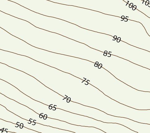
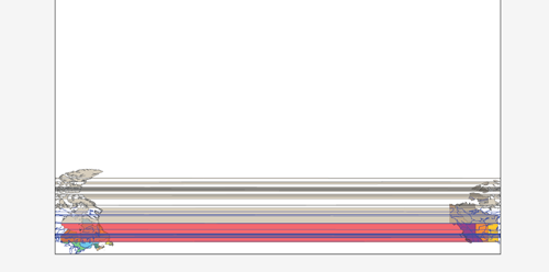
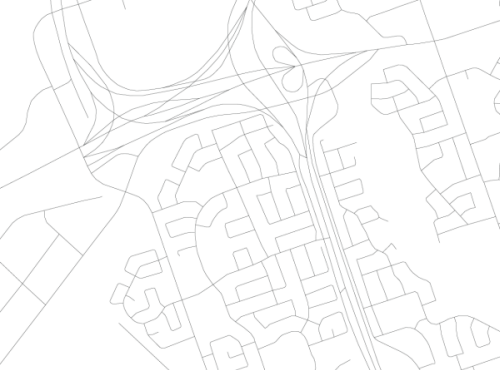
Here’s a question we receive at Avenza support quite often: I’ve located and imported a GIS layer of road lines with attributes for the city I’m mapping. How can I turn this:
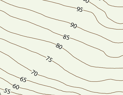
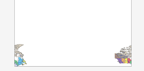
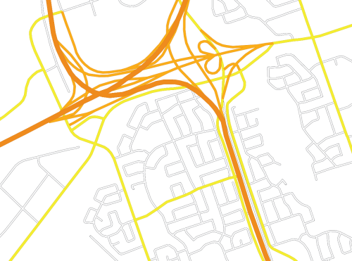
into this:

Getting Started

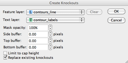
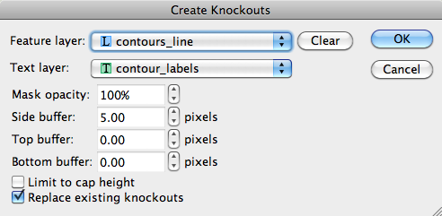
The workflow for this process involves the use of both MAPublisher and Adobe tools, specifically MAP Stylesheets and MAP Selections along with Illustrator’s Graphic Styles and the Appearance Panel.

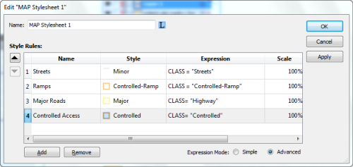
This process works on roads that have an attribute on which you can base classification rules. My road data has a column named “CLASS” with four categories: Controlled, Controlled-Ramp, Highway, and Street. I’ve created a graphic style for each and loaded them using “Open Graphic Style Library”. I keep the road styles I have created in a template document titled RoadStyles.ai so that I can import the graphic styles I need into whatever map I’m making from my template (see Adobe Graphic Styles Help).

Controlled Access Highway: Controlled Access Highway
Controlled Access Ramp: Controlled Access Ramp
Major Road: Major Road
Minor Road: Minor Road

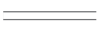
These styles all have been created using the Illustrator Apprearance panel to overlay two strokes, the top stroke with a smaller weight and different colour than the bottom stroke (see Adobe Appearance Panel Help).

With our graphic styles set I can now apply the MAP Stylesheet I built using the following expressions:

Cleaning up with groups

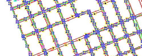
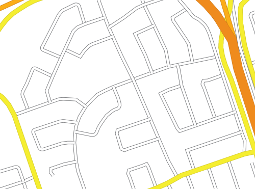
Once we apply these styles using MAPublisher Stylesheets, we will see what steps we muys take to get the appearance we want. Our roads look like this:

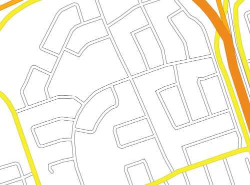
but we want them to look like this:

Why does this happen?

This occurs because MAP Stylesheets applies graphic styles at the path level. To look like intersections, each road classification must become one object, whether by being grouped or by turning the various paths into a compound path. Grouping is the preferred method for managing these objects since a compund path will delete the attributes of all paths that are being compounded. In this case, the street names field would be blank for our compound path object as dozens of streets are turned into one compund path. The consequence of this would be to make automatic labelling with MAPublisher Label Pro impossible. A set of paths turned into a group will not have their attributes available to MAPublisher while in a group, however these objects can always be ungrouped making individual paths and their original attributes available again.

Grouping Objects

In order to group our road classes we will have to select the road paths belonging to each class. The expressions we created when defining our MAP Stylesheet rules are available to us to use again through the Expression Library (new in MAPublisher 8.3). We can use MAP Selections to individually select each of our road classes. Once selected the street classes can be grouped using CTRL+G on your keyboard or Object > Group from the menu (See Adobe Group Help). The final step is to re-apply the graphic style appropriate to each group using the Adobe Graphic Style panel.

If we want to get technical here in considering what has happend to our artwork, using the Appearance panel we can see that each of the paths we initially imported now has a graphic style applied to it on two levels: at the path level (done through MAP Stylesheets) and at the group level (done by grouping and applying a graphic style to the group). It is possible to symbolize our artwork even further, at the layer level, by slecting the target symbol for our roads layer (See Adobe Layers Help). If desired we could apply a transparency at the layer level that would supersede all graphic styles used on objects in the layer. Our artwork will now have symbolization that suggests intersections, giving our road map a much neater appearance.

Tweaking

Now that our roads are grouped together, they are much easier to manage in the Illustrator Layers panel.

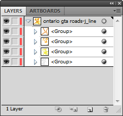
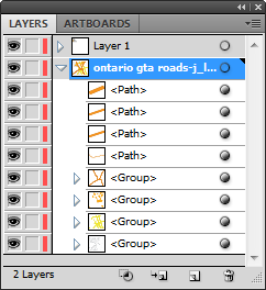
Groups can be stacked easily. My preference is to arrange with minor roads at the bottom, increasing to multi-laned divided highways at the top of the hierarchy. With our objects grouped it is easy to move objects between groups. Any path can be selected using the Direct Selection Tool and dragged in the Layers panel between groups. This is much simplier than having to use the Appearance panel to strip the path of both graphic styles and apply the desired style. There will be some situations where we will need to override the intersection appearances that result from grouping. In this image we have onramps that definitely do not interesect as this line work suggests!

To do this we must select the road lines that will be on top of the intersection, and using the Illustrator Layers panel, drag them from their group (it does not matter where in the layer hierarchy the are placed).

Our ungrouped ramps can now be sent backwards and forwards relative to other paths, giving a truer representation of the road network:

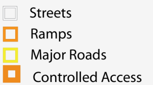
Using MAP Stylesheets to create a Legend

So why use stylesheets if we must manually group the objects after use? For a few reasons: it keeps us organized, it adds the expressions to the expression library, and most importantly MAP Stylesheets can automatically generate a Legend for us that reflects our Stylesheet rule names:

Good luck creating customized road styles! A deeper understanding of the Illustrator object styling hierarchy can go a long way in helping you use MAPublisher to leverage your GIS datasets!

Create Knockouts with MAPublisher 8.3

We receive many questions about cartographic techniques. A very popular question from MAPublisher users is “How do I mask lines behind contour labels?”

Adobe Illustrator provided some tools to achieve that through a pretty complicated workflow, so we decided to create our own tool! The upcoming release of MAPublisher 8.3 has a very handy new feature called Create Knockouts, here is how it works.

First, you need a labelled map – for example contours and labels.

No knockouts

Start the Create Knockouts tool. All you need to do is choose the layer that contains the lines to be masked and the text layer with the labels.

Create Knockouts button

There are many options available, but let’s keep the default (100% opacity, no buffer around the text, use the default text bounding box from Adobe).

Create Knockouts dialog box

The result:

Tight fit around label

These knockouts are little bit tight after all, maybe we should add some buffer distance on the side. Start Create Knockouts again (no undo required!). Choose a side buffer of 5 pixels, and make sure to check “Replace existing knockouts”.

Create Knockouts dialog box

Et voilà!

Perfect!

MAPublisher 8.3 is releasing very soon. Watch our Twitter and News page for announcements.

Avenza State Plane Coordinate System Map

MAPublisher and Geographic Imager provide an extensive library of predefined coordinate systems available for referencing or transforming mapping projects.

In the United States, the NGS (National Geodetic Survey), a department of NOAA (National Oceanic and Atmospheric Administration) has established a system that divides the United States into 124 zones, each with its own custom projected coordinate system. This system is known as the State Plane Coordinate System. It is important to note that there are two sets of State Plane coordinate systems defined in the United States, one based on the North American Datum of 1927 and the other based on the North American Datum of 1983. In addition to NAD 83, the NAD83 HARN and NSRS2007 adjustments are available for use. All three versions of NAD83 are available in metres, feet or international feet.

State Plane Coorindate Systems projections

There are four projections for SPCS. The geometric direction of each state determines the projection utilized. For states that are longer in the east-west direction, the Lambert Conformal Conic is used. States which are longer in the north-south direction use the Transverse Mercator projection. The panhandle of Alaska, which has the sole distinction of lying at an angle, garners the use of the Oblique Mercator projection, while Guam uses a Polyconic projection.

These coordinates systems are all defined in the MAPublisher and Geographic Imager library, however the initial question “which one do I need to use for my map” cannot be answered by the software itself.

There are a number of ways to determine in which zone your American area of interest lies. One online resource, searchable by latitude and longitude coordinates, can be found on this NGS website.

In an effort to better assist mapmakers in their selection of the appropriate system, the Avenza support team has prepared a searchable interactive map using MAPublisher 8.2 MAP Web Author tool. View the SPCS map here.

A MAPublisher geospatial PDF of the same map is also available for download here.

Transform into State Plane Coorindate Systems using MAPublisher

When it comes time to transform your data into the appropriate State Plane Coordinate System zone, use the MAP View Editor Perform Coordinates System Transformation option. When you specify the destination coordinate system for the transformation, navigate to Coordinate Systems > Projected > North America > United States > US State Plane NAD 83 – on the right hand list, you’ll find all the state plane zones sorted by state name and zone name: select the right one!

Note: similarly you can select the NAD27 state plane systems from Coordinate Systems > Projected > North America > United States > US State Plane NAD 27 if appropriate.

Improved Reprojection Engine in MAPublisher 8.3

One of the exciting new changes in MAPublisher 8.3 is that we’ve substantially rewritten our reprojection engine. What I’d like to do here is explain what the changes are, and what they mean for you, the user.

The old reprojection engine was point-by-point. Essentially, we walked each path and simply reprojected each point one by one. This simple approach works very well but it has one important deficiency: it lacks context. The internal reprojection system never sees anything more than a single point, and therefore is limited to just reprojecting.

So what is the new system doing? Our new reprojection engine is performed feature-by-feature. This is important because it means the internal system no longer just sees a single point, but rather a collection of points and how they are arranged. This means it can notice things like an area that wraps around to the other side of the world! In the old system, it would just blindly punch out points, and if a path suddenly jumped to the other side of the page, well, that’s where the path went. But now the reprojection engine can notice things like that, and clip the art appropriately. If necessary, it will even break a single path into a compound path! But it’s probably easier to understand if we demonstrate it visually.

Here is a map of Canada with two layers: rivers & provinces. Both sets of art are coloured nicely and the provinces layer even has an opacity reduction to make the rivers stand out a little.

Before transform

I’ve created a new coordinate system I’ve called ‘Miller Cylindrical Shifted’. I just made a copy of the ‘Miller Cylindrical’ coordinate system and then altered my copy’s central meridian to be 90 instead of zero. I did this so that if I reproject Canada into ‘Miller Cylindrical Shifted’, half of Canada should be on the left-hand side, and half should be on the right-hand side. Let’s see how MAPublisher 8.2 handles it:

After transform in 8.2

Yikes! The old reprojection engine had no idea that some of those lines were going off the end of the projection’s envelope!

Now let’s try it in MAPublisher 8.3 with the new reprojection engine:

After transform in 8.3

Wow! What a difference feature-by-feature makes! The new engine recognizes that those paths needed to be clipped and properly split polygons and lines as needed. It’s also important to note that the areas & lines are still intact. e.g. Northwest Territories was split, but it’s still a single compound path with all of its islands — some of those islands have simply been split into pieces. The split even preserves all the original path’s properties, including attributes and styles!

Import Geodatabase Feature Classes into Adobe Illustrator

In this post, we’ll cover how simple it is to import a geodatabase feature class into Adobe Illustrator using MAPublisher import tools enabled with the Spatial Database add-on.

Imported features

Spatial databases are optimized data repositories for spatial data storage and management. Many GIS environments use spatial databases to easily access and manage GIS data in a central location.

MAPublisher 8.2 introduces support for import of the popular ESRI single-user and multi-user Geodatabases: Personal, File and ArcSDE Geodatabases; and direct access to ArcSDE server. The MAPublisher Spatial Database importer is built on ESRI software libraries and requires a valid ESRI software and license installed on the computer (ArcGIS 9.2 and higher).

To import one, you can use either Simple Import or Advanced Import. In this scenario, we’ll use Advanced Import. When we add data, a list of Geodatabase types are located at the bottom of the Format list. We’ll be importing some feature classes from a simple geodatabase consisting of waterlines, hydrants and valves.

Add dialog box

After browsing for the geodatabase (a File geodatabase in this case), the Select Feature Classes dialog box appears. We’ll go ahead and select a few feature classes from the Landbase and Water feature sets listed.

Select Feature Classes

The Advanced Import dialog box shows the number of features being imported and the coordinate system as well as page and map anchors.

Confirm geodatabase import

The features are imported and are ready to be used in a map.

Imported features

Easy Transformations in MAPublisher

MAP Views are designed to provide an easy method of accessing settings for specifying and transforming coordinate systems, for editing scale and data placement on the page and for exporting to GIS formats. The MAP Views panel allows for merging Adobe Illustrator layers, georeferencing existing Adobe Illustrator artwork, changing multiple layer names, and reprojecting data on the fly.

That said, it’s possible to create multiple MAP Views that each contain a different projected coordinate system in a single map document. The MAP Views panel can be used to move Adobe Illustrator layers from one MAP View to another, enabling to reproject vector art quickly. Layers can be moved via drag-and-drop or with the new Switch MAP View button. This is useful when testing how a variety of projections may fit into your layout. It’s also useful for creating inset or key maps.

Here we have one MAP View called USA – NAD27. As the name of it implies, it is in a NAD27 projection. Let’s go ahead and make another MAP View so that we can perform an easy transformation.

USA in NAD27

Click the USA – NAD27 MAP View to highlight it, then click the panel option menu (upper right corner) and click Duplicate “USA – NAD27”.

Duplicate MAP View

This creates a Copy of USA – NAD27 MAP View. Double-click the Copy of USA – NAD27 MAP View to edit it.

Copy MAP View

In the MAP View editor, change the title to USA – Albers Equal Area in the Name box. Below you can see that it is currently in NAD27. Check the Perform Coordinate System Transformation check box and click Specify. In the Specify Coordinate System dialog box, in the Folder list, navigate to Projected > North America > United States and click United States: Albers Equal Area, meter in the right-hand pane. Click OK.

Choose Albers Equal Area

Back in the MAP View editor box, you’ll see that the Destination is updated to show the United States: Albers Equal Area projection. Click OK.

MAP View editor

The map is reprojected from NAD27 to Albers Equal Area.

Albers Equal Area projection

To reproject-on-the-fly by drag-and-drop, click the usa area layer and just drag it to the USA – NAD27 MAP View. Now you can switch back and forth between projections. You may want to duplicate the usa area layer in the Layers panel so that you can have two different projections at the same time. Remember to use the MAP View editor if you want to move a MAP view to retain spatial referencing.

Back to NAD27

To learn more about MAP Views, view Chapter 4 of the MAPublisher user guide.

News Archive

Blog Archive

April 2025 (1)
March 2025 (1)
February 2025 (1)
January 2025 (1)
December 2024 (2)
November 2024 (2)
October 2024 (1)
September 2024 (2)
August 2024 (2)
July 2024 (2)
June 2024 (1)
May 2024 (2)
April 2024 (2)
March 2024 (2)
February 2024 (1)
January 2024 (1)
December 2023 (1)
November 2023 (2)
October 2023 (2)
September 2023 (1)
August 2023 (1)
July 2023 (3)
June 2023 (1)
February 2023 (1)
January 2023 (2)
December 2022 (1)
November 2022 (2)
October 2022 (2)
September 2022 (1)
May 2023 (1)
August 2022 (2)
July 2022 (1)
June 2022 (2)
May 2022 (1)
February 2022 (1)
January 2022 (2)
August 2022 (1)
December 2021 (3)
November 2021 (5)
October 2021 (1)
September 2021 (3)
August 2021 (2)
July 2021 (1)
June 2021 (2)
May 2021 (2)
April 2021 (2)
March 2021 (3)
April 2021 (1)
February 2021 (1)
January 2021 (1)
November 2020 (1)
October 2020 (1)
June 2020 (2)
May 2020 (1)
April 2020 (3)
March 2020 (2)
December 2019 (1)
November 2019 (2)
September 2019 (1)
August 2019 (1)
July 2019 (1)
June 2019 (3)
May 2019 (4)
April 2019 (2)
March 2019 (1)
February 2019 (2)
January 2019 (3)
December 2018 (2)
November 2018 (1)
October 2018 (1)
September 2018 (1)
August 2018 (1)
September 2018 (1)
August 2018 (3)
July 2018 (2)
June 2018 (1)
July 2018 (1)
June 2018 (4)
May 2018 (1)
April 2018 (2)
March 2018 (4)
February 2021 (1)
February 2018 (1)
January 2018 (1)
November 2017 (1)
October 2017 (2)
August 2017 (2)
July 2017 (1)
March 2017 (1)
February 2017 (2)
January 2017 (2)
November 2016 (1)
January 2017 (1)
November 2016 (1)
October 2016 (2)
May 2016 (1)
March 2018 (1)
April 2016 (2)
December 2015 (2)
June 2015 (1)
May 2015 (1)
April 2015 (2)
December 2014 (4)
October 2014 (2)
May 2014 (4)
February 2014 (1)
October 2013 (3)
April 2013 (1)
January 2013 (2)
August 2012 (1)
October 2012 (1)
July 2012 (3)
May 2012 (2)
January 2012 (2)
August 2011 (1)
July 2011 (2)
June 2011 (2)
May 2011 (2)
March 2011 (1)
February 2011 (1)
January 2011 (5)
December 2010 (1)
November 2010 (1)
December 2010 (1)
November 2010 (1)
October 2010 (1)
August 2010 (4)
July 2010 (2)
June 2010 (3)
May 2010 (2)
April 2010 (2)
March 2010 (2)