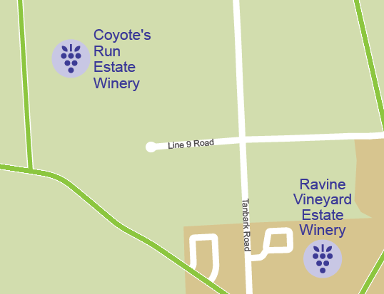
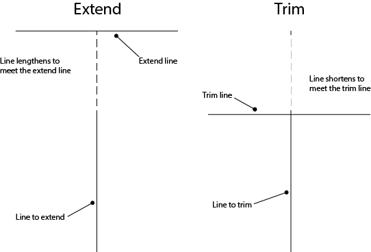
The latest release of MAPublisher includes the ability to trim and extend objects to a crossing or intersecting path. Extending a path lengthens it to meet the edge of a crossing object and trimming a path cuts the portion that extends past the edge of an intersecting path. Trim and extend tools are commonly used in CAD software and will greatly improve the ability to produce accurate and precise data in MAPublisher and clean-up imported data.
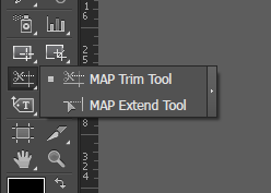
Location of the Trim and Extend tools on the Adobe Illustrator Tools panel. Click and hold the tool button to switch between MAP Trim Tool and MAP Extend Tool.
The MAP Trim Tool and MAP Extend Tools are located on the Adobe Illustrator Tools panel. Click and hold the MAP Trim or Map Extend tool button icon to switch between them. To use the tools, select the crossing or intersecting path and click the object to extend or trim. The diagram below illustrates the basic process.
Visualization of the trim and extend processes
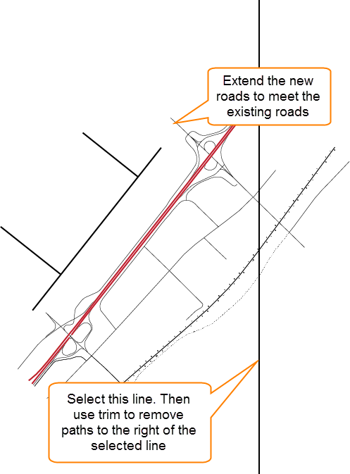
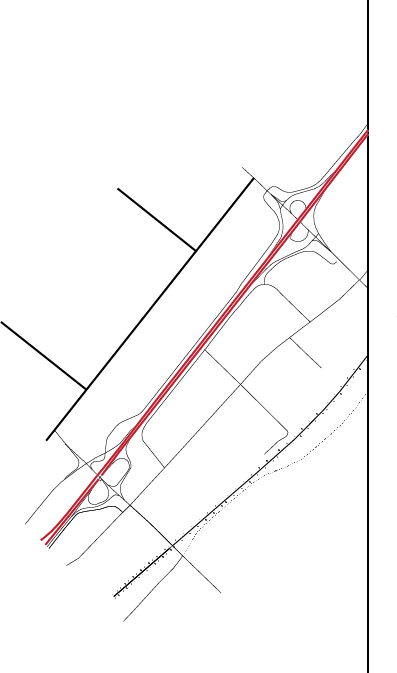
There are many possible applications for these tools in digitizing and cleaning map data. In a hypothetical example illustrated below, we trim all the roads that extend past the edge of a border, and extend the imported roads (in bold) to meet the existing roads.
Examples of uses for the trim and extend tools. Extending imported roads to match existing roads and trimming lines that fall outside of a map borderLines trimmed and extended!
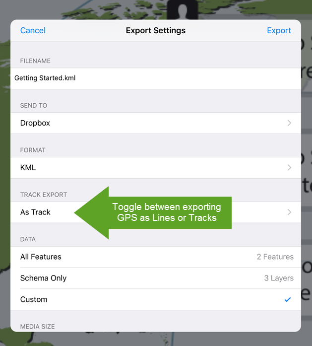
There are two methods of exporting GPS tracks from Avenza Maps in KML format: as a line and as a track. Which option to select depends on the intended purpose. Lines are much simpler than tracks and store only the position of each vertex in the line as latitude longitude and elevation. Tracks contain a complete description of how the path moves through space including the position at one-second intervals, the time at which each position was recorded, the compass angle of the heading, and the velocity. Lines take up much less storage space than tracks. To switch between exporting to Lines or Tracks, select Track Export in the Export Settings screen.
Export Settings screen
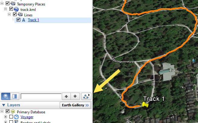
Tracks are useful in applications where the GPS position at a given time and space is important. For example, in Google Earth there is an option to record a tour that moves to predetermined places on the globe. This would be useful if you wanted to follow along on a hiking path or do a virtual walkthrough of a proposed building development. To make a tour from a track, open the KML file in Google Earth, select the track in the places panel, and click the Play Tour icon. The animation below shows a walk through Mount Pleasant Cemetery in Toronto, Canada. Lines contain only the location information: latitude longitude and elevation. Export to line when the time data is not important such as if you are making a map of a hiking trail.
Play tour in Google EarthA tour of Mount Pleasant Cemetery in Toronto, Canada using Google Earth
KML Code for Lines and Tracks
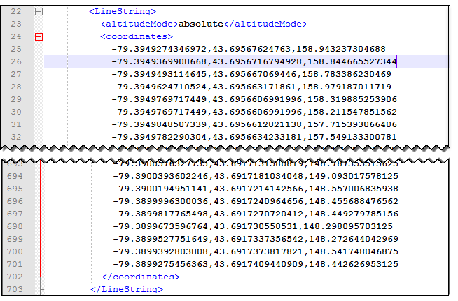
KML (short for Keyhole Markup Language) is an XML notation for displaying spatial data in web applications. It was developed for use with Google Earth and can be read by many programs. Avenza Maps uses KML to import and export placemarks, lines, and tracks. You can view and modify KML files in any text editor. The KML element used for lines is called a Linestring which is defined as “a connected set of line segments”. A Linestring element contains a coordinates tag which is a list of longitude and latitude positions in decimal degrees and elevations in meters.
KML Linestring code sample
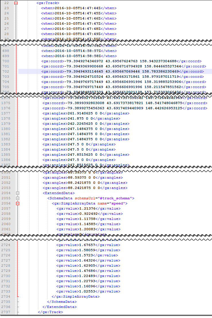
Tracks use the KML element “gx:Track” which contains several tags.
when – the date and time a point was recorded in UTC
gx:coord – the location of the point in decimal degrees and the elevation in meters
gx:angle – the current heading in compass degrees (i.e. 0 degrees is north, 90 is degrees east and so on)
gx:value tag defined as “speed” – the current speed in meters per second
There are equal numbers of each of these tags. A full description of the vertex includes all the tags in the same sequence. For instance, the first when tag, coord tag, angle tag, and speed tag, describe the first vertex in the track.
With the latest release of MAPublisher 9.9, it’s now possible to easily import layers directly from an ArcGIS Online account or an ArcGIS web service. This will allow you to use shared data layers within your ArcGIS Online organizational account and connect to publicly available map servers from various online sources.
ArcGIS Online is a collaborative web GIS that allows you to store and share GIS data using Esri’s secure cloud. Before, you may have had to download layers as shapefiles to your local machine and then import them into Adobe Illustrator using MAPublisher. Now, MAPublisher has a much improved workflow to get ArcGIS Online layers into Adobe Illustrator will full georeferencing, all map features, and attributes.
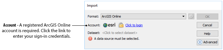
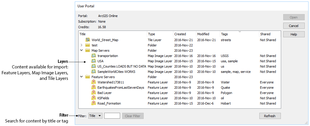
Currently, the types of datasets allowed are Feature Layers, Map Image Layers and Tile Layers. To load a layer, use MAPublisher Import as you would with any data type and select ArcGIS Online from the Format drop-down menu. Click the login link to enter your ArcGIS Online credentials to access your organization’s web portal.
Import ArcGIS Online dialog boxArcGIS Online user portal
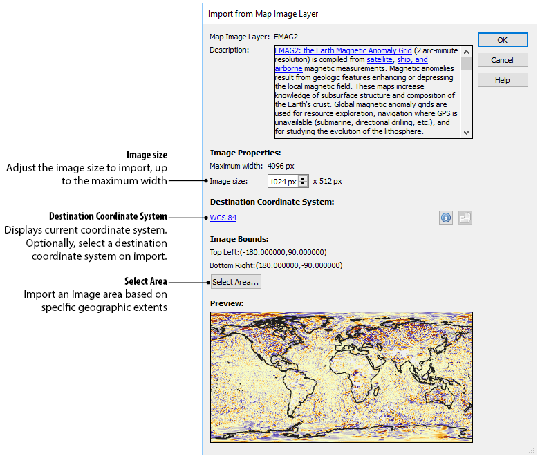
Feature Layers contain vector data that will import as artwork into Adobe Illustrator. Optionally, you can extract specific features using standard SQL queries. Map Image Layers and Tile Layers are raster data layers that can be added by selecting the geographic extents.
Import Image Map Layer
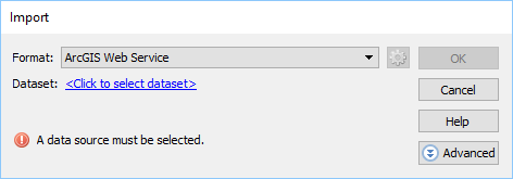
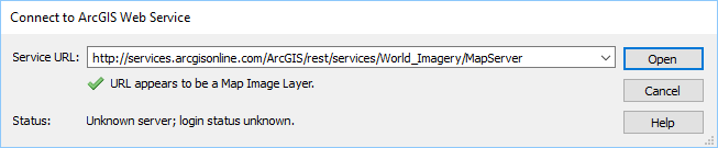
In addition to using your own organization’s data, you can connect to publicly available data from a wide variety of organizations by connecting to an ArcGIS Web Service. To connect to a web service, use MAPublisher Import and select ArcGIS Web Service from the Format drop-down menu. Click to select the dataset and enter the URL for the service. This is a great option when searching for data from open data portals created by government agencies.
Import ArcGIS Web ServiceValid ArcGIS Web Service
Accessing Esri’s online services through MAPublisher provides a great opportunity to use shared data within your organization and access a wide variety of publicly available data. We’re sure you’ll find it very useful for finding data to make great maps.
MAPublisher Grids and Graticules is a powerful tool. There are dozens of settings to create an indexed grid, measured grid, or graticule exactly the way you want. We often receive questions about how to create certain grid and graticule styles and this was interesting. We were asked how to create a graticule to display a very specific latitude and longitude, perhaps even by itself (only a single line of latitude or longitude).
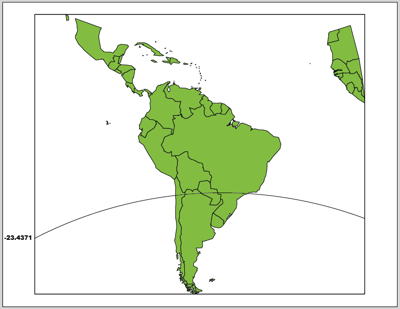
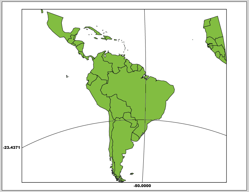
Creating a single graticule line
In this example, we’re going to create a graticule that will only display the Tropic of Capricorn at -23.4371 degrees (or 23.4371 degrees south of the equator).
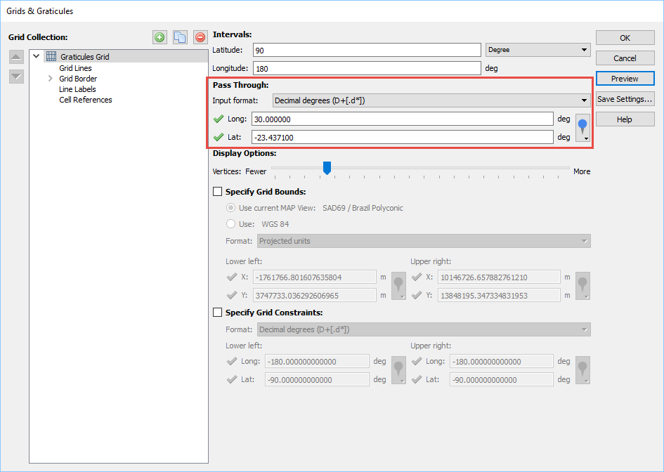
On the MAPublisher toolbar, click the Grids and Graticules button to open the dialog box. Click the Graticules button to create one. On the Graticules Grid main settings, the important setting to note here is the Pass through section — it specifies lines of latitude and longitude that must be included in the graticule. Enter 30 deg Long and -23.4371 deg Lat. This means that a graticule line must pass through -23.4371 degrees latitude (the Tropic of Capricorn). The reason why a line at 30 deg longitude is specified is to hide it from the map view (it is placed at 30 deg longitude outside of the map extent).
Pass through setting
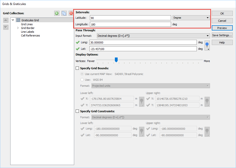
In the Intervals section, set 90 deg Latitude interval and 180 deg Longitude interval. Because the intervals are at the extreme, this means that the the only lines left to display are the ones specified in the Pass through section (30 deg long and -23.4371 deg lat). In this case, it will only display a single line of latitude (the Tropic of Capricorn) for the graticule.
Intervals setting
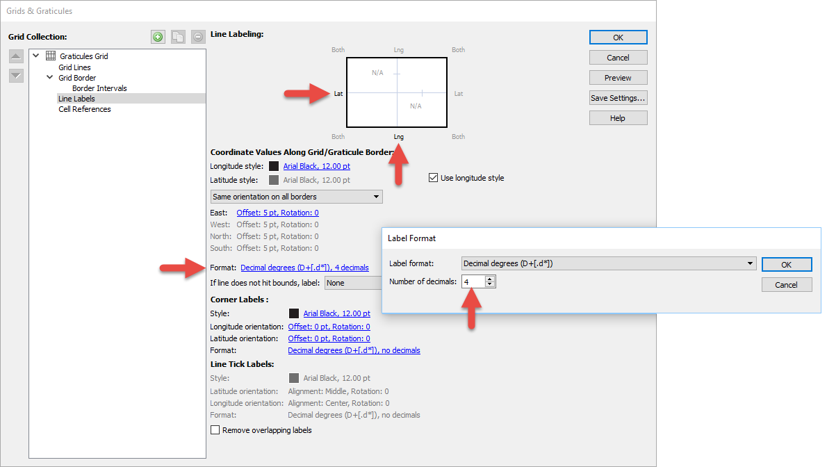
If you want to label the graticule, go to the Line Labels setting. Click the Lat and Lng on the grid label control to enable them. To control how many decimals are displayed, click the Format setting, then change the number of decimals to something greater than 0.
Label settings
To intersect single lines of longitude and latitude, adjust the Pass through setting so that the line is within the map’s extent. In this case, it was set to -50 deg (50 deg west).
Intersect single lines of longitude and latitude
Remember that you can share Grids and Graticules settings with anybody by clicking the Save Settings button, selecting a destination folder and sharing the configuration files.
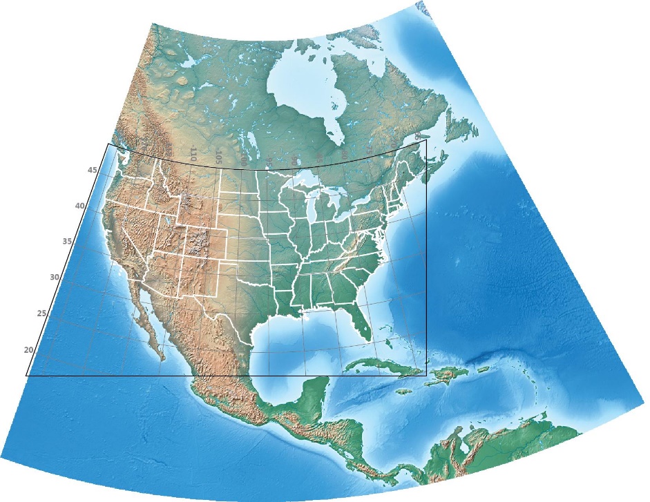
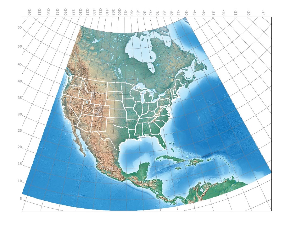
A graticule is the network of lines of latitude and longitude drawn at regular intervals on a map. Graticules are created in MAPublisher using the Grids and Graticules tool. In some maps, you may want to limit the area on the map that a graticule covers. For example, you may want it to cover only the map’s area of interest. The image below is a map of North America with a graticule drawn at 5-degree intervals. US State boundaries are drawn in white. In this post, we’ll modify the graticule three times so it conforms to the edges of the image, so it covers only the Continental United States, and lastly a combination of the previous two modifications.
North America with a graticule of 5 degree intervals.
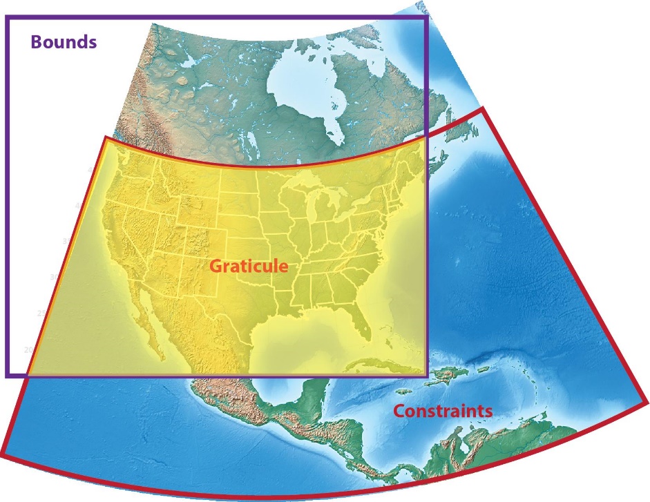
MAPublisher can limit the geographic extents of a graticule in two ways: using Grid Bounds and using Grid Constraints. In both cases, you’ll specify the lower left and upper right corners of the graticule. Specifying Grid Bounds will limit the extent of the graticule to a rectangular area while specifying Grid Constraints will limit the graticule along lines of latitude and longitude. If both Grid Bounds and Grid Constraints are specified, the graticule will cover an intersection of the two areas. The image below shows bounds and the constraints and the intersecting area which forms the graticule.
Bounds and the constraints and the intersecting area which forms the graticule.
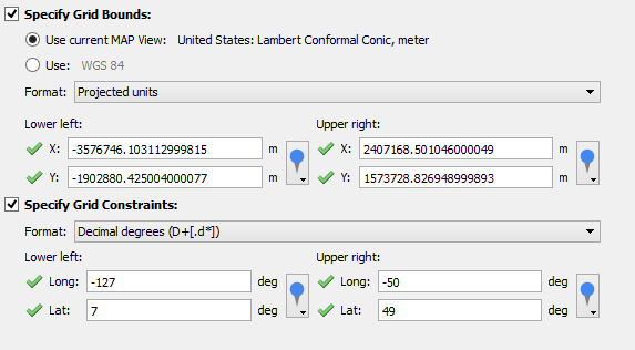
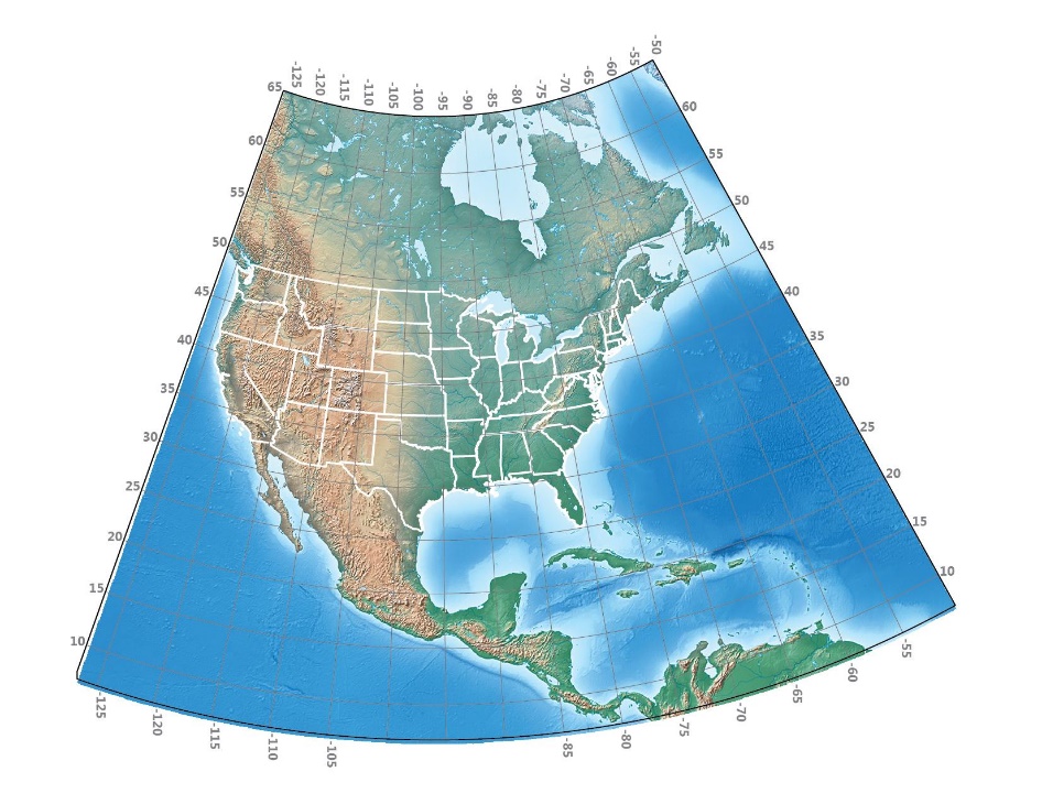
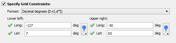
To modify a graticule so that it conforms to the edges of the image, you’ll need to specify grid constraints. In the Grids and Graticules dialog box, click the Specify Grid Constraints check box and set the Lower Left and Upper Right corners to the corners of the image which are -127°, 7° and -50°, 65° respectively.
Specifying Grid Constraints.
To create a rectangular graticule covering only the lower 48 states, click the Specify Grid Bounds check box and set the Lower Left and Upper Right corners to the corners of that area. Tip: click the MAP World Locations drop-down arrow to choose the values for the lower left and upper right corners.
Specifying Grid Bounds.
When both Specify Grid Bounds and Specify Grid Constraints check boxes are both checked, the graticule will cover an intersection of each of the extents. For instance, in the map below, the northern extent follows the 49th parallel at the Canadian border, the western extent is at the edge of the image (127° west) and the south and east extents are the same as in the previous map.
Both Specify Grid Bounds and Specify Grid Constraints selected.
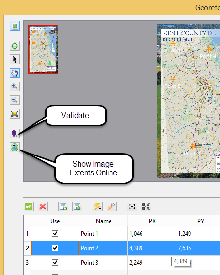
When georeferencing a map in Geographic Imager, there are two tools which can be used to check spatial accuracy: Validate and Show Image Extents Online. With Validate, click a point on the image and it will show the corresponding location on the web map service so that you can compare the difference between them. Show Image Extents Online will display a rectangle representing the spatial extent of the image on the web map.
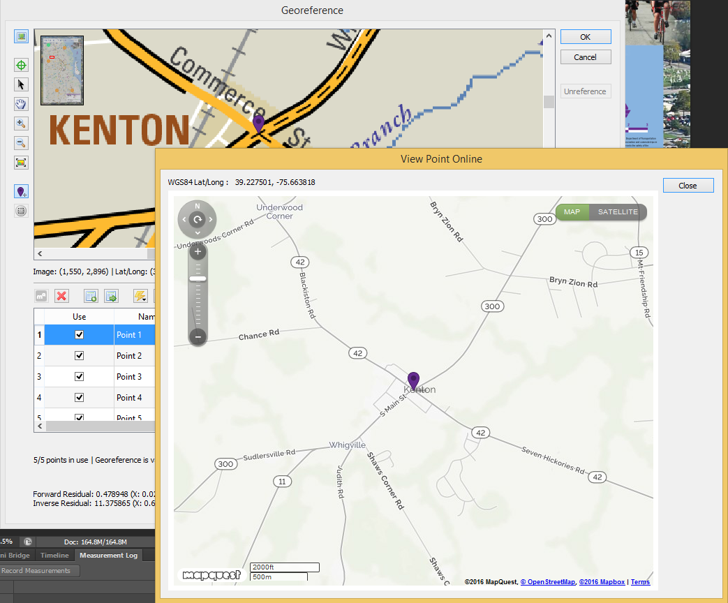
The image below shows the Validate tool in action. Selecting the tool and clicking on the road intersection brings up the same intersection in the web map, displaying how accurate the georeferencing may be. It is good practice to test several known points on the image. Choose features that will be easy to identify on the web map such as road intersections, coastlines, buildings, and landmarks.
The Show Image Extents Online tool is shown in the image below. Use this tool to see the full area covered by the image. Note that the rectangle shown on the web map will include the non-map areas of the page (borders, legend, etc).
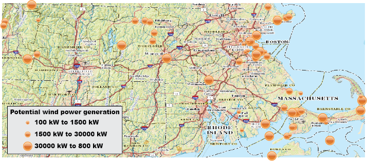
Online services can be used to create high-quality maps without the need to download and maintain large spatial datasets or spend time designing base maps. In this post, we’ll use two online sources to import data and create a map showing the potential energy generated from existing and proposed wind power projects in the state of Massachusetts.
Wind map
There are two types of online mapping services MAPublisher can use to import layers: Web Map Services (WMS) and Web Feature Services (WFS). WMS is an interface for accessing geo-registered images from an online source. This means that users aren’t able to modify individual elements of a WMS layer and are only able to select an area of the map to import. WMS also allows for transparency so map layers can be overlaid on top of one another.
WFS, on the other hand, is an interface for accessing vector map features in GML format. Features are imported as a MAP Layer which can be further modified using MAPublisher and Illustrator tools. To create this map, we’ll import data from two sources: a topo map from the US Geological Survey (USGS) and the Massachusetts Office of Geographic Information (MassGIS).
To start, open Adobe Illustrator and create a new document in portrait mode. Import a MAP Layer and select Web Feature Service from the Format drop-down. Click the “Click to select services and layer(s)”. link. The MassGIS layers are included with MAPublisher by default. If you do not see this service, click Load Services from Avenza. Select Commonwealth of Massachusetts, USA – MassGIS in the USA folder.
Selecting WFS for import
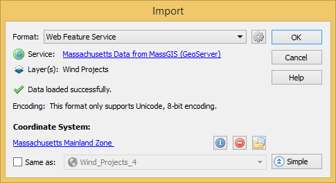
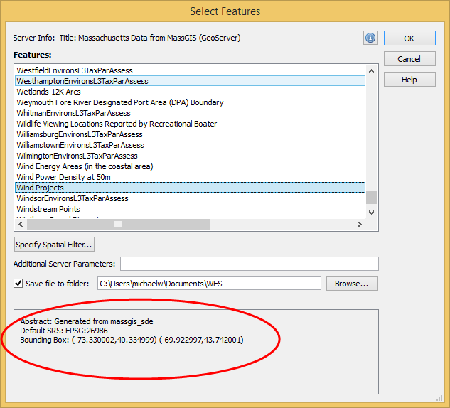
On the Select Features dialog box, select Wind Power. Note the default SRS – EPSG 26986. On the Import dialog box, click the link to select a coordinate system. Choose Massachusetts Mainland Zone (EPSG 26986). Click OK.
WFS information
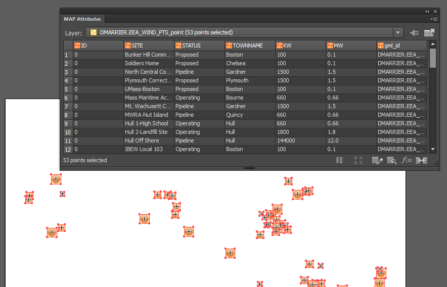
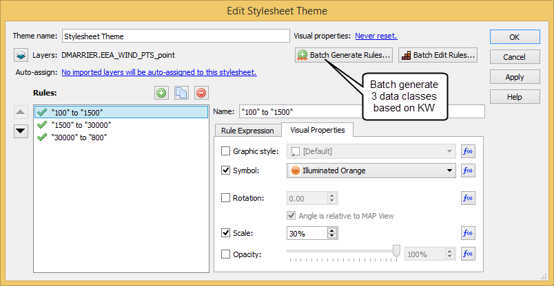
The Wind Projects layer has been imported as a MAP Layer. It can be modified using MAPublisher or Illustrator tools to symbolize, label, select, and so forth. To create the style for this layer, add a new Stylesheet MAP Theme of Point feature type, then Batch generate rules for the KW column using three quantiles, and select Set scale so the symbols scale proportionally to the value. For more on how to replicate this style, see the MAPublisher Help article MAP Themes.
Wind point attributes (click to see larger image)Batch generate rules
The next step is to import a WMS layer to use as a base layer. This map uses the USGS Topo Base Map which was created as part of the National Map program. A list of WMS and WFS services provided by USGS is available at http://viewer.nationalmap.gov/services/.
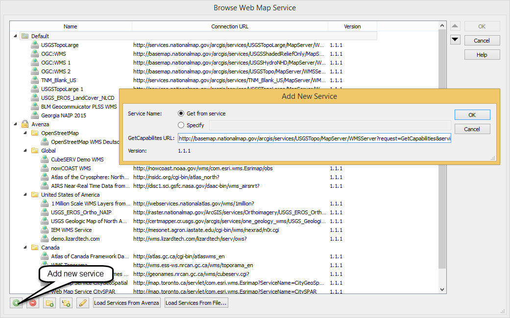
Go to the USGS web page and open the WMS link under Base Maps (Cached) > USGS Topo Base Map – Primary Tile Cache (Tiled). This is an XML document with the location and metadata of the WMS. Copy the link from the address bar and in Adobe Illustrator, click the MAPublisher Import button and choose Web Map Service from the Format drop-down menu. Click the “Click to select service and image” link. Click Add New Service and paste the URL into the GetCapabilities URL text box. Choose the service from the list and click OK.
Add new service
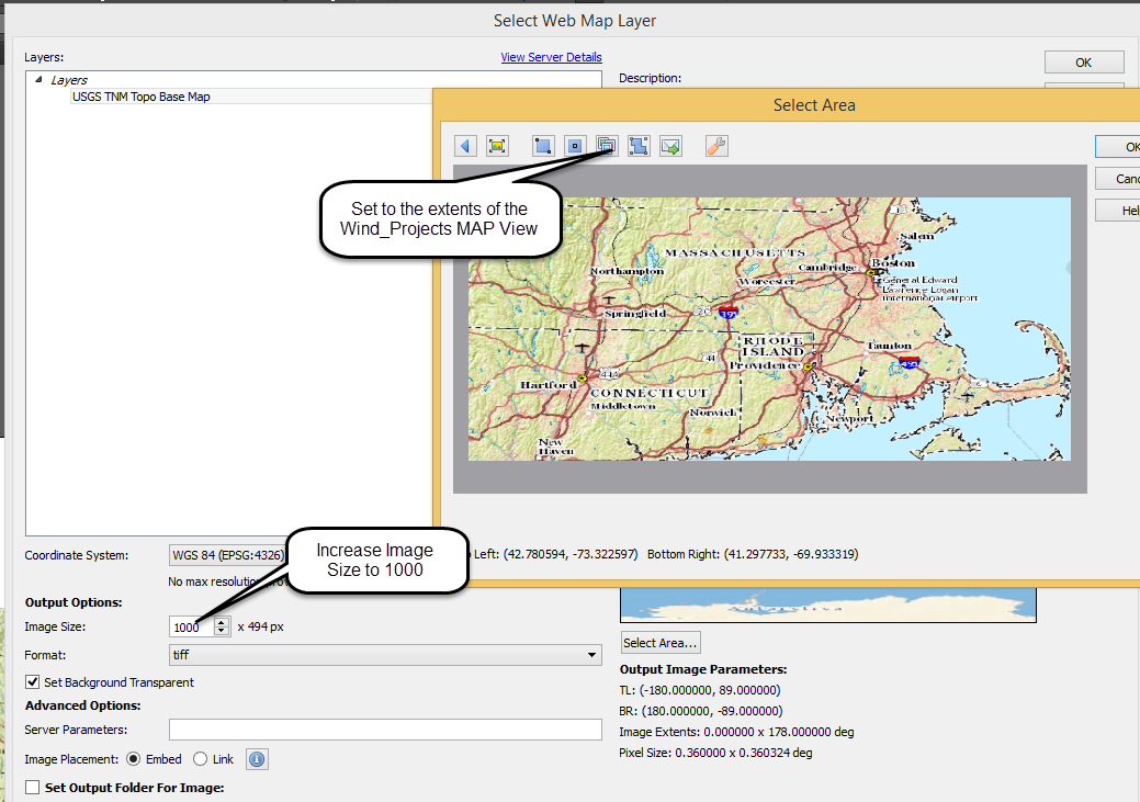
On the Select Web Map Layer dialog box, choose USGS Topo Base Map from the Layers list. Set the Image Size to 1000 to increase the resolution. To change the extents of the output image click Select Area. This dialog box provides several options for setting the extents of the base map image. Click-and-drag to specify an area to select – the image will automatically crop. The buttons at the top of the panel allow you to enter the coordinate extents manually, match the extents of a MAP View or match the extents of a vector layer. Since we have already added the Wind Power layer to the map, we will set the extents to match this map view by clicking “Select area by MAP View” and choosing Wind_Projects from the drop-down menu. Leave the other options as default and import the base map image.
Select area
For the final step, open the MAP View panel and drag the layer DMARRIER.EEA_WIND_Point to the MAP View USGS_TNM_Toppo_Base_Map. This will transform the points to the same coordinate system as the base map.
There are thousands of freely available WMS and WFS sources available online. For a good starting place see this blog post from the Open Geospatial Consortium for advice on finding services. You could also use a basic web search – for example – “WMS Toronto” or similar. For more help on web services in MAPublisher see the help article Web Map/Feature Service.
March 3rd is National Cold Cut Day… so happy #NationalColdCutDay to you! Cold cuts have been around for more than 2,000 years and today, it is so ubiquitous that any populated place with a market or grocery store stocks it. Even more so, the up-rise of fast food provides the convenience of someone making a cold cut sandwich for you (even better!). Recently, we came across a subreddit called /r/subwaysubway – a collection of subway-style maps of Subway® sandwich restaurants. While most cities boast several dozen Subway locations, Toronto, ON has the density and population to support more than 200. So in honour of National Cold Cut Day, we’re going to create a Subway subway map of Toronto with some of our favourite mapping tools. While this is only meant to be a light-hearted project and not an authoritative source of all Subway locations, please forgive us if we missed a few locations. That said, we used some available web tools in combination with MAPublisher to create a mapping workflow that might inspire you to create your own Subway subway map.
Finding Subway locations
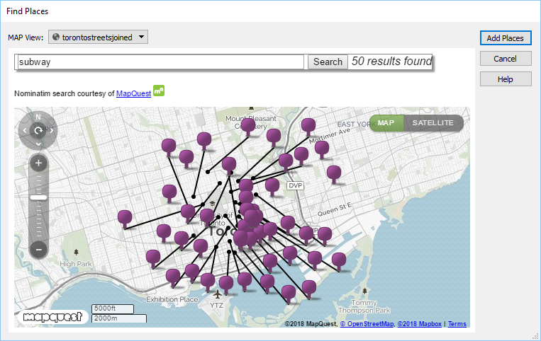
Finding all (most) of the Subway shops was easier said than done. A combination of several sources were used to achieve this. We used the MAPublisher feature called Find Places to scan areas of Toronto to search and import the Subway location point data. This task was performed several times, simply because of the high density of Subway locations in Toronto. In addition, the source provides useful attribute data including name, address, and neighbourhood fields that will be useful for labeling (more on that below).
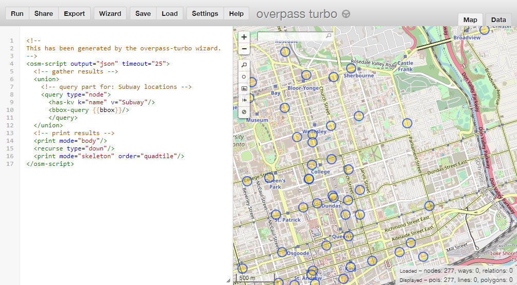
To verify these locations, we also used a web tool called overpass turbo that has some handy tools to build a query that searches OpenStreetMap and filters data that can be easily exported. We simply exported the queried locations as a KML file and used MAPublisher to import it. Unfortunately, these locations did not include any attribute data, however, there were several points included that the MAPublisher Find Places tool missed. We then searched Google Maps and the Subway website to verify several addresses that were missing in the attribute data. Again, we probably missed some locations, but this is supposed to be fun, right?
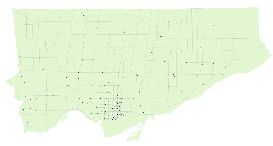
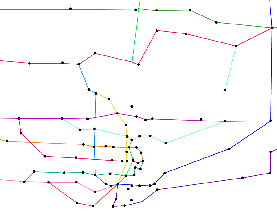
With most of the sourcing completed, we end up with a map that looks like the one below. All the Subway restaurant locations can now be considered subway stations. We also used a Toronto boundary layer and streets layer from Open Data Toronto that was transformed to use a projection of NAD 83 / UTM Zone 17N with a -18 degree rotation at approximately 1:65,000 scale. The boundary and streets layer won’t be used in the final map, but helps when navigating the map, especially if you’re (un)familiar with the city.
Converting to a subway style map
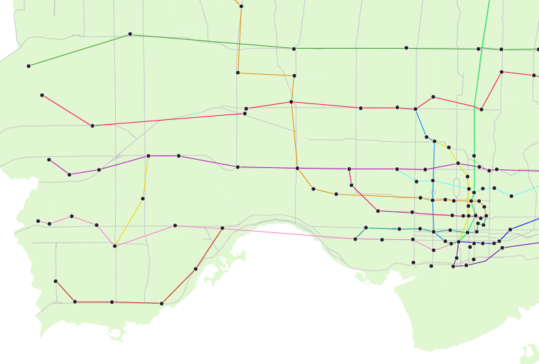
Using a very liberal amount of cartographic license, we created MAP line layers and used the Adobe Illustrator pen tool to connect Subway locations to what felt natural based on knowledge of the city including following major roads, existing transit corridors, geography, and neighbourhoods. The downtown core was the most difficult to connect as it was densely populated with Subway shops (almost one at every major intersection — impressive), although it loosely represents the grid layout that the downtown core is actually based on.
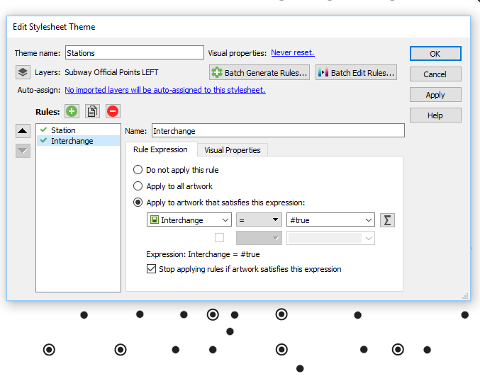
After some quick connections, we created a MAP Theme to style for the Subway points layer. We created two styles: one for regular stations and one for interchange stations – where our fictional subway riders (eaters?) can transfer to another line. To mark stations as an interchange, we created a new boolean attribute that designates it as true or false. If the rule is true, then it uses a Interchange symbol to denote it as an interchange.
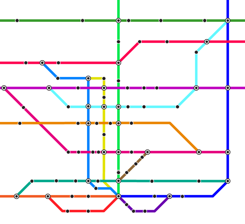
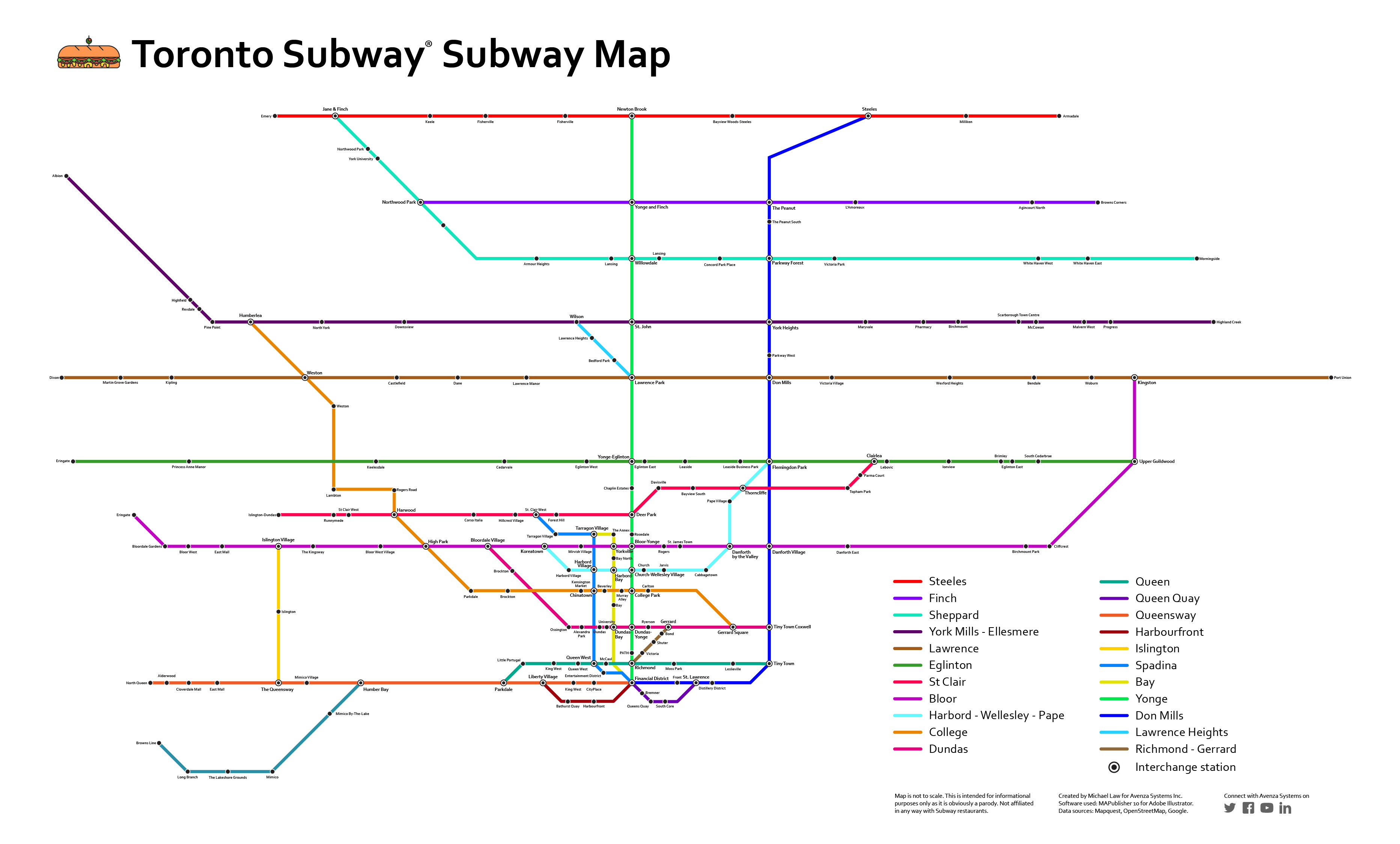
Once we felt like we had a solid coverage with interconnecting lines, we copied the Adobe Illustrator document to a new one, hid the boundary and street layers, and began the task of converting it into a styled subway map. For simplicity, we used a typical orthogonal method that employs lines at any multiple of 45 degrees. Needless to say, this took some time and patience as there are many points to align, nudge and decipher. This is where having the geographically accurate map, some of the online maps, and other sources to refer to was very handy.
Compare it to the geographic version (some lines and points may have been moved or redone during the conversion to follow the orthogonal method).
Labeling shouldn’t be tough, right?
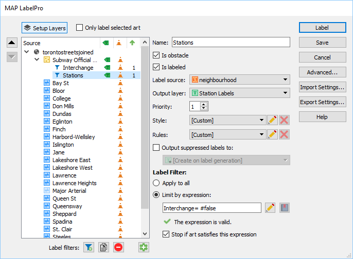
We decided to use MAPublisher LabelPro, an intelligent and obstacle-detecting labeling engine, to label the subway stations because there are so many of them. With a little bit of setup, it can label the entire map in just a few seconds. Using the same rule used to designate stations as an interchange, we created two styles for the labels using the label filter. Interchange stations are slightly larger and have a bold font. We designated the label source to use the attributes from the Subway point layer, in this case, a neighbourhood name. Lastly, we designated the lines as obstacles so that LabelPro can detect whether a label will interfere with them or not.
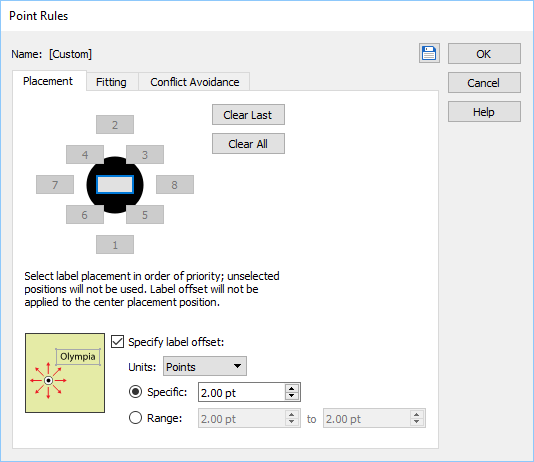
We also configured placement rules so that the stations have a preference to be labeled at bottom and top, and then at positions around the point if the first two aren’t possible. In addition, we specified a label offset so that the labels are placed more evenly without too much fine-tuning afterwards.
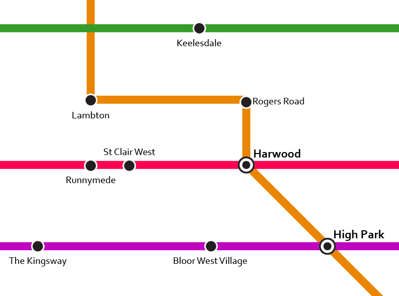
After LabelPro placement and some manual tweaking, the result is a cleanly labeled map. Here’s a detailed view.
While the neighbourhood attribute was unique in most cases, some dense areas such as downtown Toronto had station names repeat itself. In these instances, we relabeled them with its street name, a nearby landmark or park. This may not be the most accurate, but it was fun to come across neighbourhoods or areas we’ve never heard of and it allowed us to learn more about our own city. Another great source to use was this Toronto neighbourhood map that allowed us to quickly verify which neighbourhood a particular Subway sandwich was in.
While we’re sure there are probably many more tweaks to make to this map and more stations to add, here’s our take on the Subway subway Map of Toronto. Make sure to click the links below to see the high-res PDF versions.
Avenza desktop applications, MAPublisher and Geographic Imager offer two options for the licensing system: Fixed license and Floating license.
The Fixed license option allows only one license per computer. For most users or small companies, this is generally sufficient, even with a few licenses. Since your license is fixed to a specific computer, it can’t be moved freely to another machine. However, Avenza does allow you to move your license occasionally. For example, if you purchased a new computer or when your computer is being fixed and you need to transfer your fixed license to another computer. If your subscription status for MMP (MAPublisher Maintenance Program) or GMP (Geographic Imager Maintenance Program) is up-to-date, then moving your fixed license to another computer (i.e. rehosting a license) can be done without a cost. Complete this form to do so. You will receive a notification email from Avenza when this is completed.
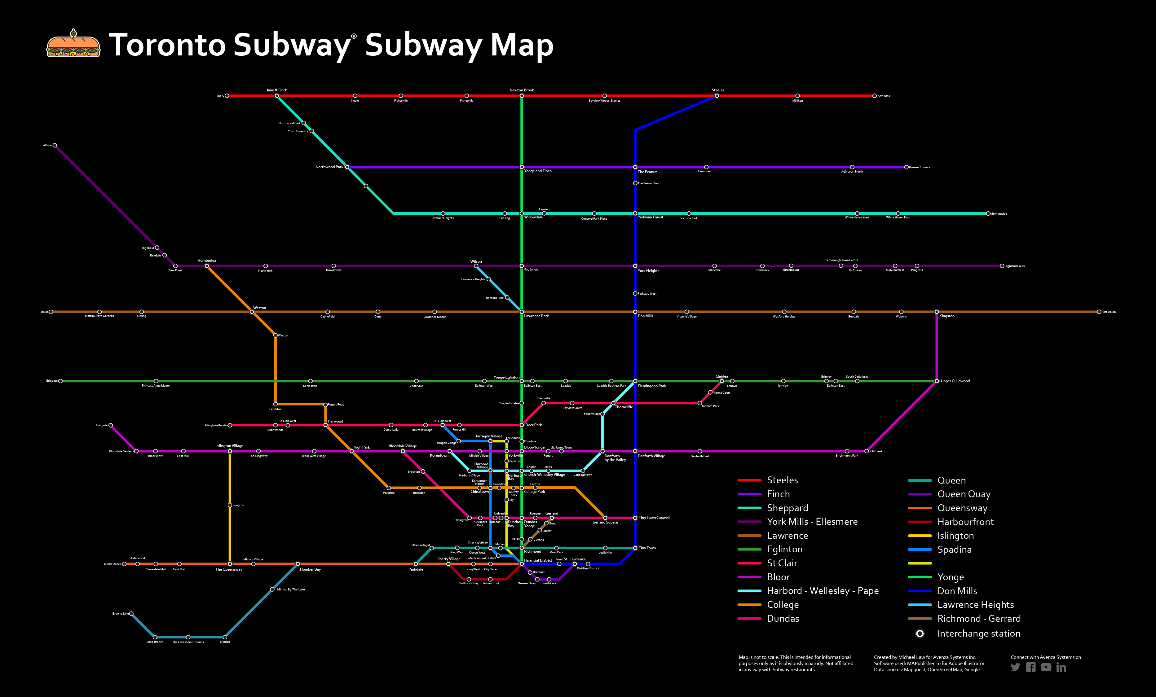
The Floating license option is for users who wants to share a number of licenses on the network. This is a great solution for any size company that has multiple users who share use of MAPublisher or Geographic Imager. You will need to set up a license server for which users will need check out a license from the server before using MAPublisher or Geographic Imager. In general, this option is used when sharing a number of license with colleagues. For example, the license server holds two seats of MAPublisher license. When users on Computer A and Computer B are using MAPublisher, other users can’t check out a license until the borrowed licenses are checked in.
Another great advantage of the floating license the ability to borrow a roaming license with their laptop so that they can use MAPublisher and Geographic Imager outside their immediate office. This is a good solution for users who need to use the software on the go and doesn’t have a connection to the floating license server.
For more information about the licensing options for our MAPublisher and Geographic Imager, contact Avenza sales.
If you have any technical questions about setting up a license server or any other licensing issues, contact Avenza Technical Support.
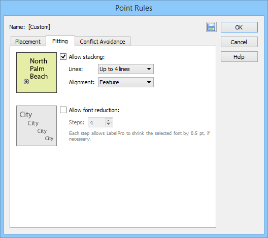
There may be times when you want to have labels be multiple lines. Multi-line labels allow them to fit in tighter positions on the map. Currently, in MAPublisher LabelPro there’s a rule to allow stacking up to 2, 3 or even 4 lines. However, this rule only “allows” stacking and doesn’t “force” stacking. It is only meant to fit labels when there isn’t enough space for a single line.
MAP LabelPro allow stacking rule
Fortunately, there is a trick to manually force text to label as multi-line: you need to manipulate the text attribute. Always make sure to create a backup or duplicate of your layer before trying this on your own data.
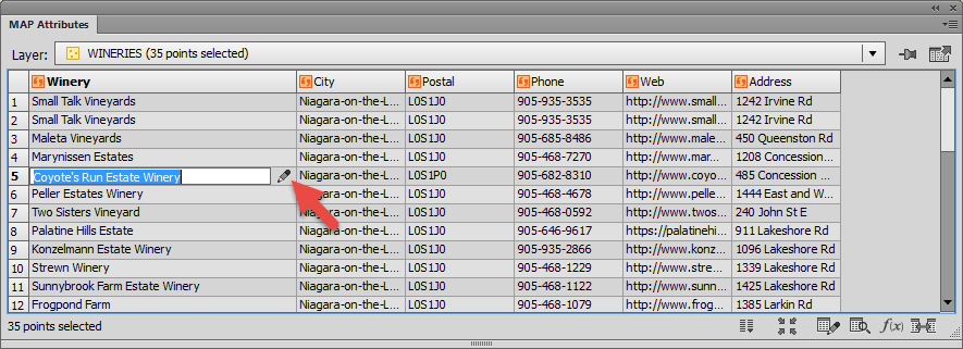
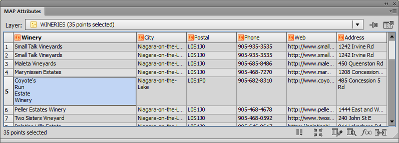
1. Go to your attribute table. Double-click to edit the text and click the Edit icon.
Edit feature attribute in MAP Attribute table
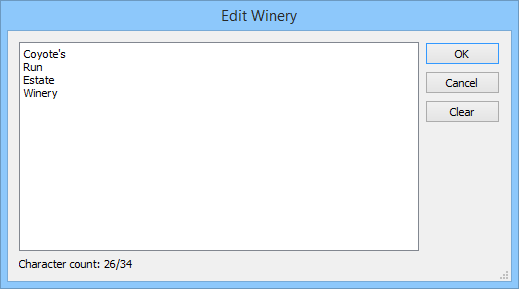
2. Edit the text so it is on separate lines.
Edit the text so it is on separate lines
In the attribute table, you will only see the first word of the multi-line text. But all the text is still there and you can see it by adjusting the row height.
Adjust the row height to see all the text
3. Run MAPublisher LabelPro, Label Features, or the MAP Label Tagger tool. MAPublisher will label the feature using the multi-line text specified in your attributes.
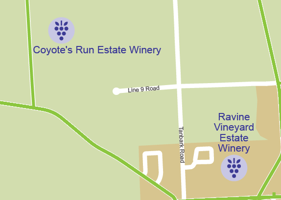
Labeling result
If you have the Allow Stacking rule enabled in MAPublisher LabelPro, it won’t affect multi-line text since it’s already setup that way. Generally, it’s good practice to leave the allow stacking rule enabled in case other labels require tighter fitting. Remember to create a MAP Text layer to contain labels that could not be placed. This can provide hints as to what LabelPro rule adjustments you need to make.


 To create a rectangular graticule covering only the lower 48 states, click the Specify Grid Bounds check box and set the Lower Left and Upper Right corners to the corners of that area. Tip: click the
 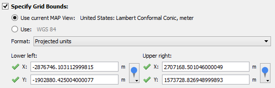 When both Specify Grid Bounds and Specify Grid Constraints check boxes are both checked, the graticule will cover an intersection of each of the extents. For instance, in the map below, the northern extent follows the 49th parallel at the Canadian border, the western extent is at the edge of the image (127° west) and the south and east extents are the same as in the previous map.